Analytic Fog Rendering With Volumetric Primitives

In this post I’m going to cover a neat technique for rendering regions of fog with varying density. I’ll start by covering some of the basic principles behind fog rendering and a few common solutions before describing the technique itself. There will be a bit of maths involved – you’ve been warned!

A Brief Review of Fog Rendering

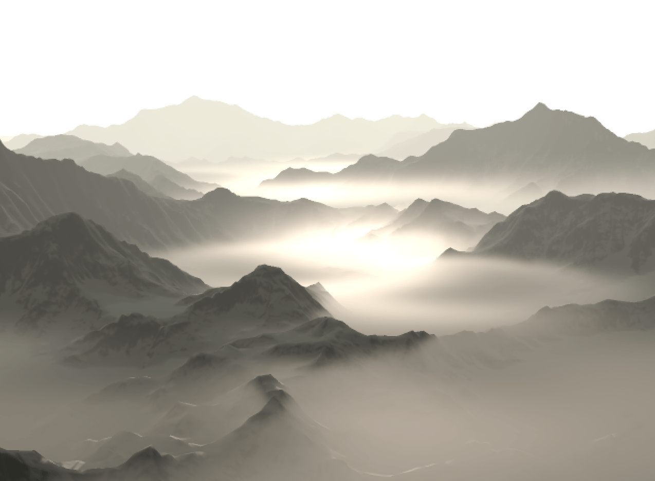
For those unfamiliar, rendering fog boils down to simulating the behaviour of light as it passes through a medium. The simplest behaviour we can model and the one we’re going to focus on is absorption, or the loss of light energy. In basic terms, the more ‘stuff’ that light has to pass through, the more energy it loses.

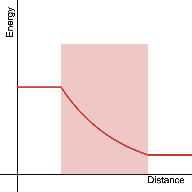
A light ray loses energy as it travels through a medium (shaded region).

The ratio of outgoing light to incoming light after a given ray passes through a medium is called the transmittance, its value $T$ defined as:

$T = \dfrac{L_o}{L_i}$

Where $L_i$ is the amount of light entering the medium and $L_o$ is the amount coming out. The relationship between the density of the medium and transmittance is described by the Beer-Lambert Law. The equation is:

$T = e^{-\tau}$

Where $\tau$ is the total density encountered by the light path going through the medium. Once we have the transmittance, we can just multiply it by $L_i$ to find out how much outgoing light reaches us through the ray. If the medium is just an area of constant density $\rho$ , then $\tau$ simply evaluates to the length $\ell$ of the portion of the light ray passing through the medium times the density:

$\tau = \rho \ell$

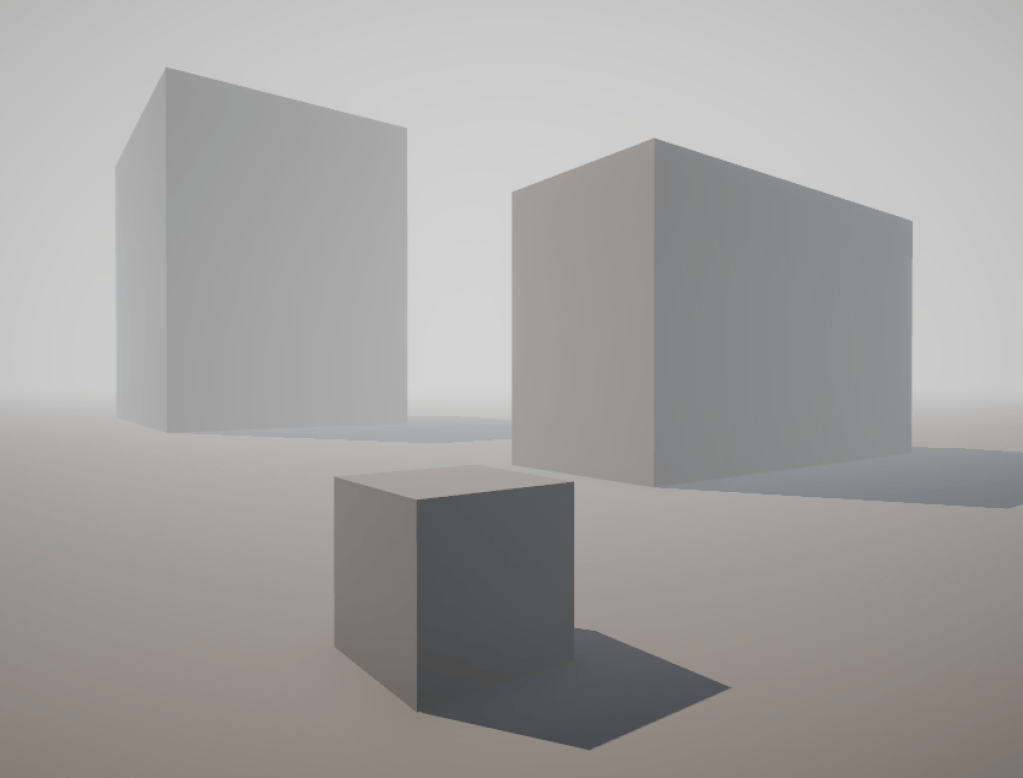
This is more or less the approach the approach used to render simple distance fog in games. Sometimes the Beer-Lambert Law is foregone completely and just the total density $\rho \ell$ along the ray is used to fade objects in the distance. Either way this approach not only assumes a medium of constant density, but that the medium itself covers the entire viewable area.

An example of basic exponential distance fog.

By constraining our medium within a bounded region we can give ourselves a bit more flexibility on the appearance of fog within a scene. The simplest approach is to use primitives such as planes, spheres or boxes as bounding volumes. By determining the intersection of our view ray with these primitives we can find the length of the ray through the volume and calculate the total density $\tau$ using the same formula, once again assuming a constant density within the entire primitive.

Spheres, boxes, and planes can be used to bound regions of fog.

I won’t cover ray-primitive intersection here as it’s beyond the scope of this post and there are loads of resources describing efficient algorithms to do this already. Inigo Quilez has a number of great examples on how to implement these on his website.

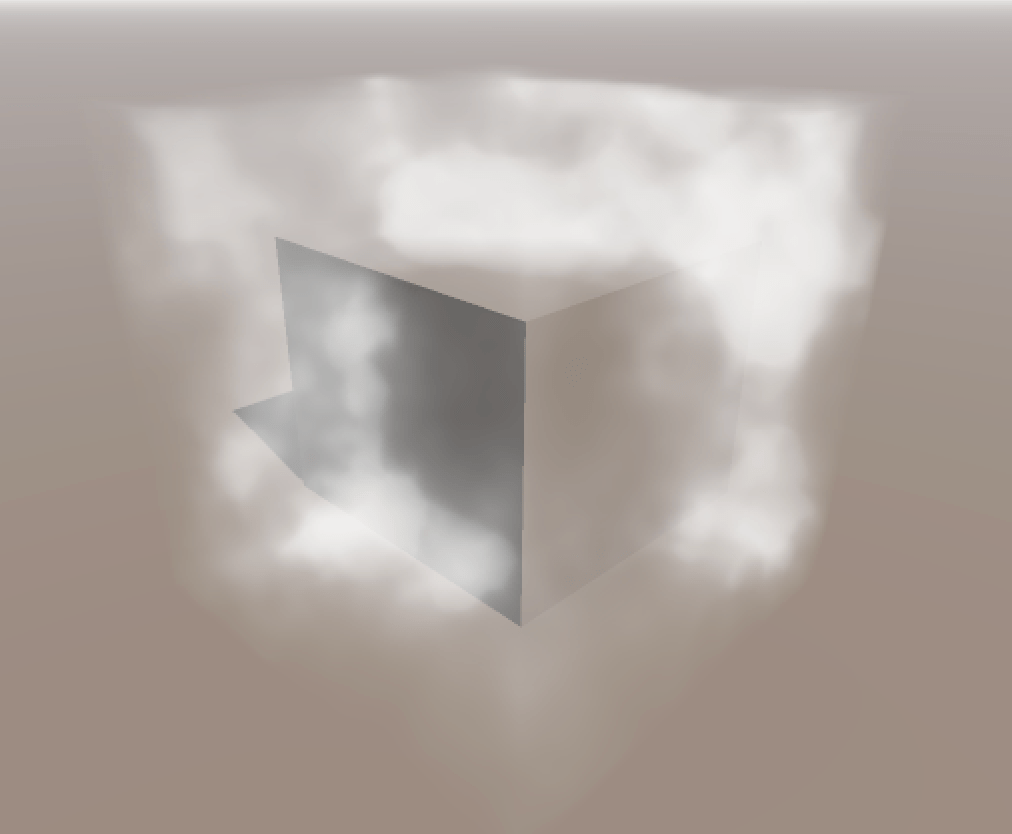
Heterogenous Volumes

In reality it’s rare that we can take a medium’s density as constant throughout its entire area, especially when it comes to clouds or smoke. When a medium has a non-constant density we say that it is heterogenous. A greater range of effects can be simulated if we take this into account when rendering. Unfortunately this can complicate the equation quite a bit. Now $\tau$ is no longer a simple product but an integral over the light ray:

$\begin{aligned} \tau = \int_{t_a}^{t_b} f(p) \,dp \end{aligned}$

Here, $t_a$ and $t_b$ are the start and end points of the portion of the ray passing through the bounding volume, respectively. The function $f(p)$ describes the density of the medium at a given point in space $p$ . Because not all functions have a closed-form solution for their integral, we often resort to numerical methods to evaluate it, i.e. moving along the ray in small steps and adding up the area of rectangular ‘slices’ of density along the way.

The integral of an arbitrary function can be approximated by adding up the area of lots of small rectangular slices.

This is effectively what ray-marching does and is pretty much the bread and butter of modern volume rendering. It’s extremely flexible – we don’t care what the density function is, and in fact we may not even know what it is, but as long as we can sample it at arbitrary points (e.g. via a volume texture) we can numerically evaluate the integral.

Ray-marching can be used to render volumes of fog with varying density.

Ray-marching does have its drawbacks however, most notably in the form of aliasing as a result of using too few samples to approximate the integral. While analytic solutions are less flexible, they will never alias and are often faster to compute, which is good motivation for finding analytic expressions for different types of media.

Radial Functions

A function that depends on the distance of some point $p$ relative to the origin can be considered a radial function. These are nice as they’re often simple to work with and let us define volumes where the density varies over a region. By combining many of these radial density functions we can create more complex fog- or smoke-like effects.

Many radial density functions can be combined to create regions of fog with varying density.

Getting the integral along a line segment is not too difficult for simple functions. Recall that a radial function is dependent on the distance of a point $p$ to the centre, which for the sake of simplicity we’ll take to be the point at zero. So the distance is simply:

$\|p\|$

The equation for a point on a ray with origin $r_o$ and direction $r_d$ at a distance $t$ is given by:

$p = r_o + tr_d$

So the distance to any point along the ray can be expressed as:

$\|r_o + tr_d\| = \sqrt{(r_o + tr_d)\cdot(r_o + tr_d)} = \sqrt{at^2 + 2bt + c}$

Where:

$a = r_d \cdot r_d, \quad b = r_d \cdot r_o, \quad c = r_o \cdot r_o$

For a given radial function we can rewrite it in terms of $\sqrt{at^2 + 2bt + c}$ to get a new function that we can (hopefully) integrate. For a more intuitive visual understanding, consider the new function as one that describes the change in density through a cross-section of the original function.

The integral along a ray can be interpreted as the area under the cross-section of the density function (shaded region).

We can apply linear transformations to the ray origin $r_o$ and direction $r_d$ to place arbitrary scaled and rotated volumes anywhere in space without having to change any of the following calculations. This is done by multiplying the ray equation by a transformation matrix $M$ in the following way, yielding the transformed ray origin and direction $r^{\prime}_o$ and $r^{\prime}_d$ :

$r^{\prime}_o +tr^{\prime}_d = M(r_o + tr_d) = Mr_o + tMr_d$

All that’s left is to find the antiderivative of our new function and evaluate it at the limits corresponding to the start and end of the ray. If $F(p)$ is the antiderivative of $f(p)$ , then:

$\begin{aligned} \tau = \int_{t_a}^{t_b} f(p) \,dp = F(t_b) - F(t_a) \end{aligned}$

However, it’s possible that we run into issues with numerical precision when the ray origin is far away from the primitive. We can fix this by moving $r_o$ to the beginning of the interval at $t_a$ , then setting new limits at 0 and $t = t_b - t_a$ , reducing the equation to:

$\begin{aligned} \tau = \int_{0}^{t} f(p) \,dp = F(t) - F(0) \end{aligned}$

Now I’m going to go through a few radial functions and find the antiderivative of the density along a given ray. You know – for fun!

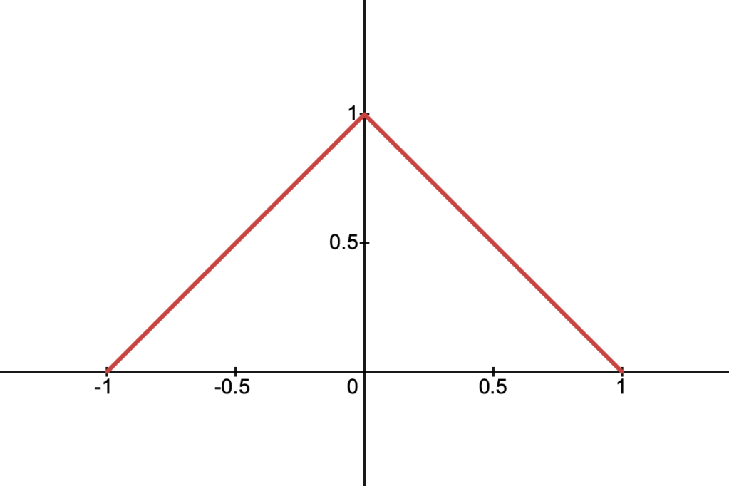
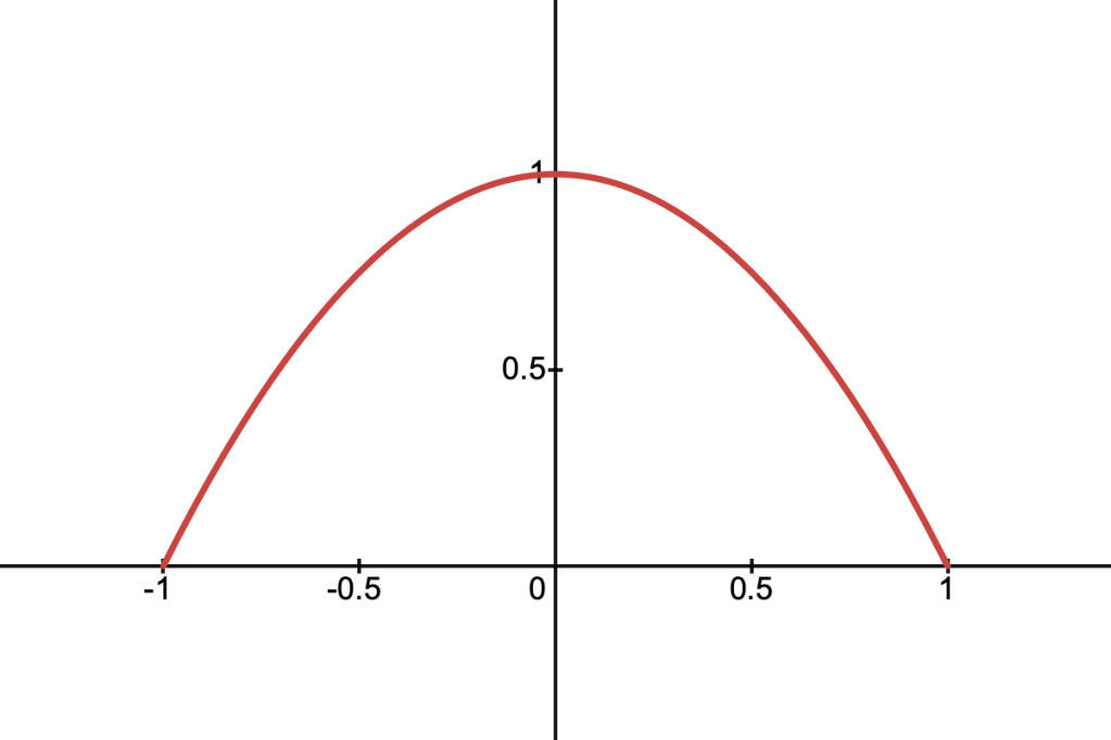
Linear Density

This function corresponds to a triangular function in 1D or a cone in 2D. It’s described by the following equation:

$f(p) = 1 - \|p\|$

Using the same logic as above, we can define the function for the density along an arbitrary cross-section, which we’ll call $\bar{f}(t)$ :

$\bar{f}(t) = 1 - \sqrt{at^2 + 2bt + c}$

To find the antiderivative $F(t)$ start by pulling out the constant $a$ and completing the square:

$\begin{aligned} F(t) &= \int 1 - \sqrt{at^2 + 2bt + c}\,dt \\ &= t - \sqrt{a} \int \sqrt{t^2 + \dfrac{2b}{a}t + \dfrac{c}{a}}\,dt \\ &= t - \sqrt{a} \int \sqrt{\left(t + \dfrac{b}{a} \right)^2 - \left(\dfrac{\sqrt{b^2 - ac}}{a}\right)^2}\,dt \end{aligned}$

Then by setting:

$u = t + \dfrac{b}{a}, \quad v = \dfrac{\sqrt{b^2 - ac}}{a}, \quad du = 1 \,dt$

We can use the following identity:

$\begin{aligned} \int \sqrt{u^2 - v^2} \,du = \dfrac{1}{2} \left(u \sqrt{u^2 - v^2} - v^2 \ln{|u + \sqrt{u^2 - v^2}|}\right) + C \end{aligned}$

Which gives us the final equation, still using $u$ and $v$ for brevity:

$\begin{aligned} F(t) = t - \dfrac{\sqrt{a}}{2} \left(u \sqrt{u^2 - v^2} - v^2 \ln{|u + \sqrt{u^2 - v^2}|}\right) + C \end{aligned}$

It might be a good idea to add a small offset to the value inside the logarithm, avoiding precision errors near 0. Here’s what all that looks like in code:

float antiderivativeLinear(float a, float b, float c, float t)
{
    float u = t + b / a;
    float v = (b * b - a * c) / (a * a);
    float radical = sqrt(u * u + v);

    return t - sqrt(a) * (u * radical - v * log(0.001f + u + radical)) / 2.0f;
}

Quadratic Density

This function resembles a parabola and is described by:

$f(p) = 1 - \|p\|^2$

Its cross-section along a ray is given by:

$\begin{aligned} \bar{f}(t) &= 1 - (at^2 + 2bt + c) \\ &= -at^2 - 2bt - c + 1 \end{aligned}$

Which is nice because we don’t have to deal with any square roots. The equation is a quadratic polynomial in $t$ and the antiderivative is easy to solve for:

$\begin{aligned} F(t) &= \int -at^2 - 2bt - c + 1\,dt \\ &= -\dfrac{a}{3}t^3 - bt^2 - (c + 1)t + C \end{aligned}$

float antiderivativeQuadratic(float a, float b, float c, float t)
{
    return t * (t * (t * a / -3.0f - b) - c + 1.0f);
}

Quartic Density

This function is given by:

$f(p) = (1 - \|p\|^2)^2$

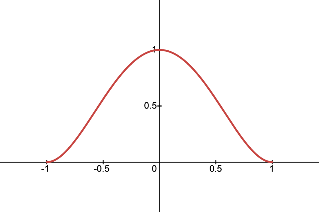
And its cross-section along a ray is:

$\begin{aligned} \bar{f}(t) &= (1 - (at^2 + 2bt + c))^2 \\ &= a^2t^4 + 4abt^3 + 2(2b^2 + ac - a)t^2 + 4(bc - b)t + c^2 - 2c + 1 \end{aligned}$

This function is particularly nice because its derivative is zero at the boundaries, similar to smoothstep. The cross-section is a quartic polynomial in t, and the antiderivative is also easy to find:

$\begin{aligned} F(t) &= \int a^2t^4 + 4abt^3 + 2(2b^2 + ac - a)t^2 + 4(bc - b)t + c^2 - 2c + 1\,dt \\ &= \dfrac{a^2}{5}t^5 + abt^4 + \dfrac{4b^2 + 2ac - 2a}{3}t^3 + 2(bc - b)t^2 + c^2t - (2c - 1)t + C \end{aligned}$

float antiderivativeQuartic(float a, float b, float c, float t)
{
    return 
        t * (t * (t * (t * (a * a * t / 5.0f + a * b) + 
        (2.0f * b * b + a * c - a) * 2.0f / 3.0f) +
        (b * c - b) * 2.0f) + (c * c - 2.0f * c + 1.0f));
}

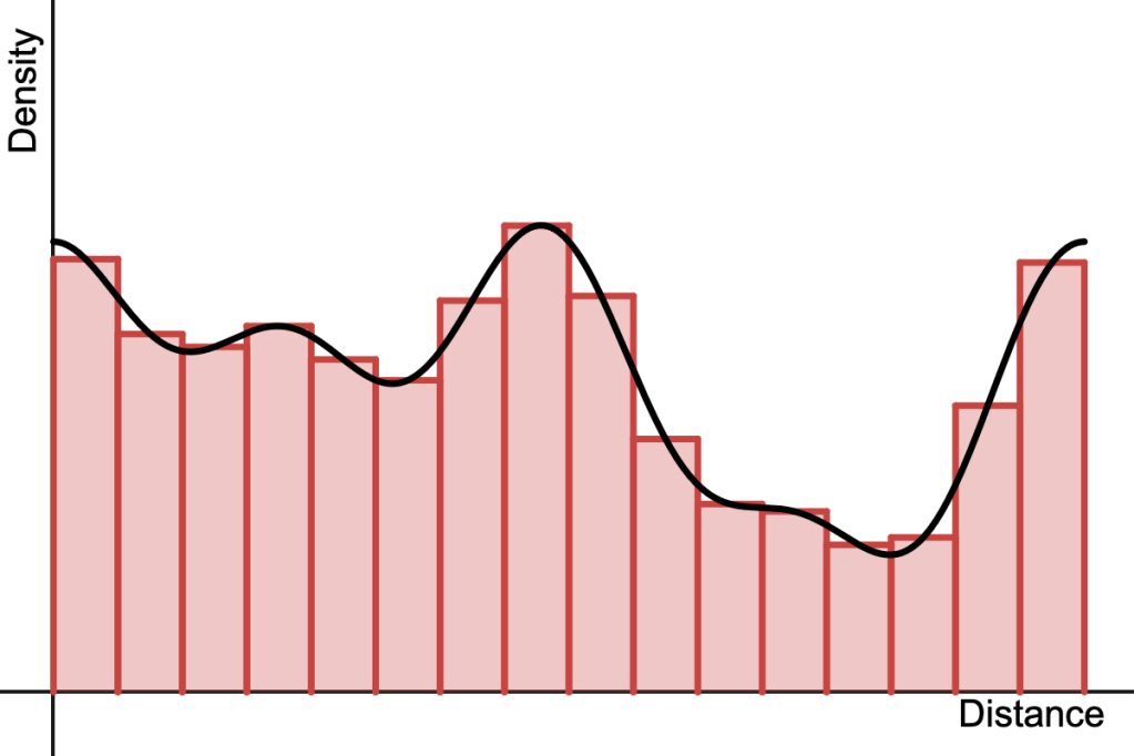
Spiky Density

This is a density function which peaks sharply in the centre and falls off smoothly to zero at the boundaries. It’s defined as:

$f(p) = (1 - \|p\|)^2$

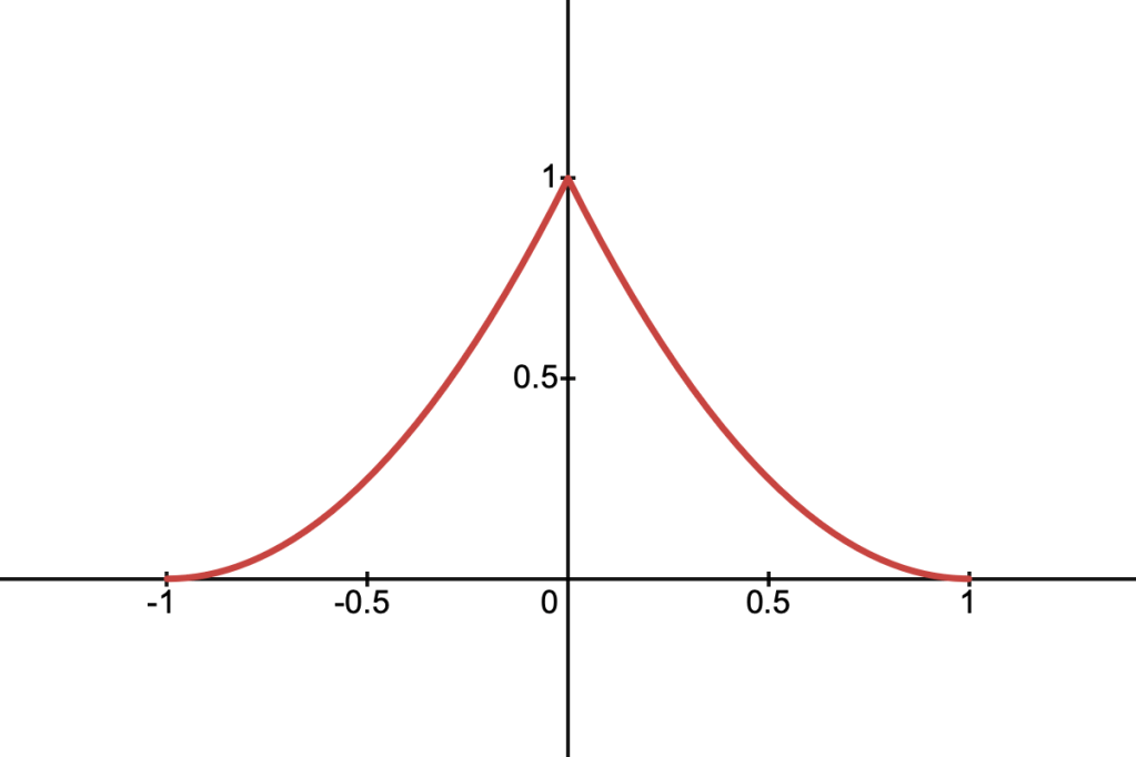
It’s cross-section is given by:

$\bar{f}(t) = (1 - \sqrt{at^2 + 2bt + c})^2$

To find the antiderivative, start by expanding out the brackets:

$\begin{aligned} F(t) &= \int (1 - \sqrt{at^2 + 2bt + c})^2\,dt \\ &= \int at^2 + 2bt + c - 2\sqrt{at^2 + 2bt + c} + 1 \,dt \end{aligned}$

We can deal with the $2\sqrt{at^2 + 2bt + c}$ term the same way we did with the linear density function. The rest of the terms are straightforward. This gives us:

$\begin{aligned} F(t) &= \dfrac{a}{3}t^3 + bt^2 + t(c + 1) - \sqrt{a} \left(u \sqrt{u^2 - v^2} - v^2 \ln{|u + \sqrt{u^2 - v^2}|}\right) + C \end{aligned}$

Where once again:

$u = t + \dfrac{b}{a}, \quad v = \dfrac{\sqrt{b^2 - ac}}{a}$

float antiderivativeSpiky(float a, float b, float c, float t)
{
    float u = t + b / a;
    float v = (b * b - a * c) / (a * a);
    float radical = sqrt(u * u - v);

    return 
        t * (t * (t * a / 3.0f + b) + c + 1.0f) - 
        sqrt(a) * (u * radical - v * log(0.001f + u + radical));
}

Gaussian Density

This is the well-known Gaussian function, defined as:

$f(p) = e^{-\|p\|^2}$

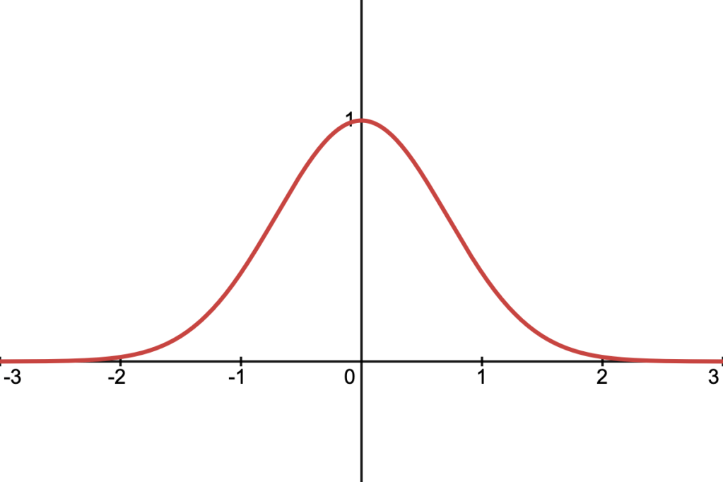
It’s cross-section along a ray is:

$\bar{f}(t) = e^{-at^2 - 2bt - c}$

To find the antiderivative we need to use a function known as the error function, defined as:

$\begin{aligned} \text{erf}(z) = \dfrac{2}{\sqrt{\pi}} \int_{0}^{z} e^{-x^2} \,dx \end{aligned}$

To start, we can complete the square in the exponent, which lets us pull out some constant terms from the main integral:

$\begin{aligned} F(t) &= \int e^{-at^2 - 2bt - c} \,dt \\ &= \int e^{-a\left(t + \frac{b}{a}\right)^2 + \frac{b^2}{a} - c} \,dt \\ &= \int e^{-a\left(t + \frac{b}{a}\right)^2} e^{\frac{b^2}{a} - c} \,dt \\ &= e^{\frac{b^2}{a} - c} \int e^{-a\left(t + \frac{b}{a}\right)^2} \,dt \\ \end{aligned}$

Now we’ll rearrange the exponent so that it’s in the form $e^{-u^2}$ :

$\begin{aligned} F(t) &= e^{\frac{b^2}{a} - c} \int e^{-a\left(t + \frac{b}{a}\right)^2} \,dt \\ &= e^{\frac{b^2}{a} - c} \int e^{-\left(\frac{at + b}{\sqrt{a}}\right)^2} \,dt \\ \end{aligned}$

Which lets us use the following substitution:

$u = \dfrac{at + b}{\sqrt{a}}, \quad du = \sqrt{a} \,dt$

Yielding:

$\begin{aligned} \dfrac{1}{\sqrt{a}} \int e^{-u^2} \,du = \dfrac{\sqrt{\pi}}{2\sqrt{a}} \text{erf}(u) + C \end{aligned}$

And after substituting back into our original equation, we arrive at the following solution:

$\begin{aligned} F(t) = \dfrac{\sqrt{\pi}}{2\sqrt{a}} e^{\frac{b^2}{a} - c} \text{erf}\left(\frac{at + b}{\sqrt{a}}\right) + C \end{aligned}$

The Gaussian is the only function we’ve covered that doesn’t fall to 0 when $\|p\| = 1$ , rather it approaches 0 as $\|p\|$ goes to infinity. In practice it’s often enough to scale $r_o$ and $r_d$ by a constant factor until the discontinuity isn’t noticeable.

// Approximation of erf.
float erf(z)
{
    float az = abs(z);
    
    return 
        sign(z) * (1.0f - 1.0f / pow(1.0f + az * (0.278393f + az *
        (0.230389f + az * (0.000972f + az * 0.078108f))), 4.0f));
}

float antiderivativeGaussian(float a, float b, float c, float t)
{
    float sqrtA = sqrt(a);

    return sqrt(PI) * exp(b * b / a - c) * erf((a * t + b) / sqrtA) / (2.0f * sqrtA);
}

Extra Stuff

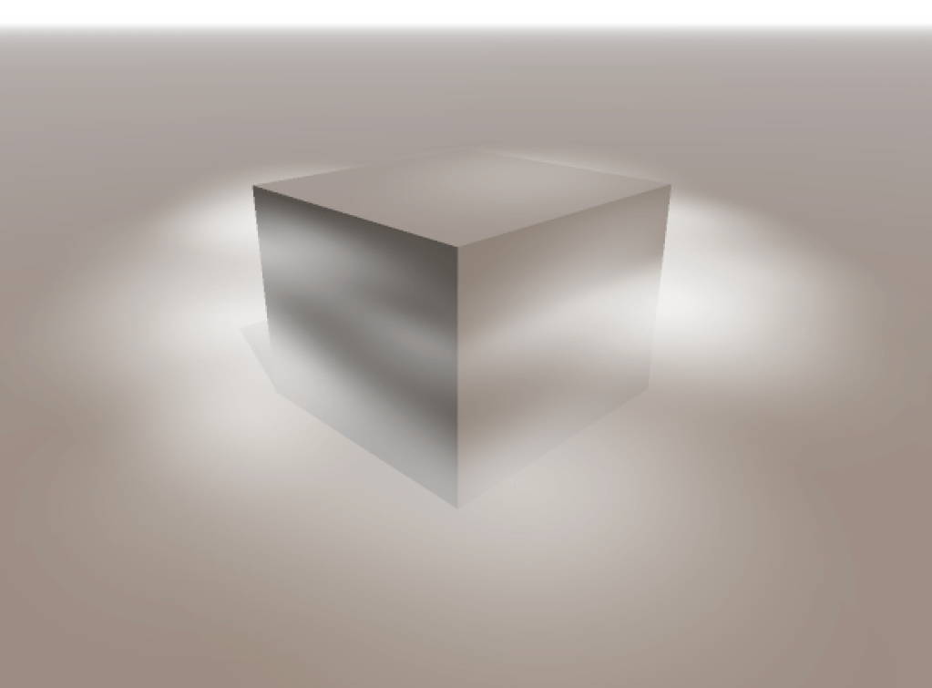
One thing I’ve left out is how to make these volumes respond convincingly to light and shadow. Unfortunately the full equation describing this physical behaviour is too complex to solve analytically. However, a quick hack is to apply a very simple shading model to each individual primitive in the hopes that, as a whole, the medium appears to react to light as we expect it to.

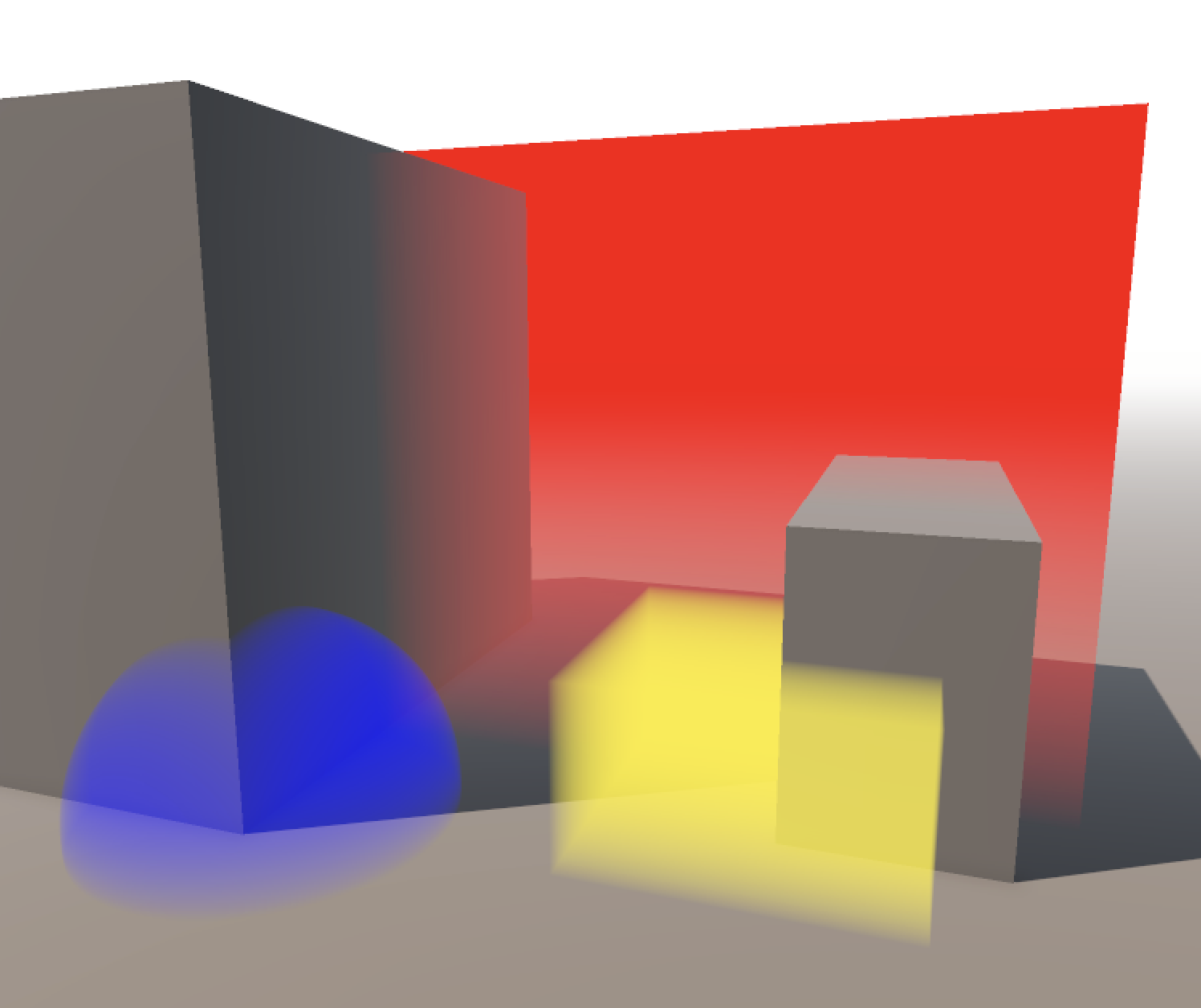
Convincing lighting effects can be achieved using a relatively simple lighting model for each fog primitive.

Representing fog as a collection of primitives opens up some neat possibilities as well. For example, it shouldn’t be too hard to hook these primitives up to a particle system to achieve dynamic or animated fog effects. If we want to be clever we can also use boolean operations to create more complex bounding volumes. This could be used to produce a simple fog of war effect for instance.

Regions of fog can be ‘cut out’ using boolean operations.

I hope you’ve found this technique interesting and find some potential uses for it in your projects. If you’d like a visualisation of all these density functions along with their source code, please take a look at this Shadertoy implementation I put together. Thanks for reading!

Analytic Fog Rendering With Volumetric Primitives

A Brief Review of Fog Rendering

Heterogenous Volumes

Radial Functions

Linear Density

Quadratic Density

Quartic Density

Spiky Density

Gaussian Density

Extra Stuff

Published by matejlou

Leave a Comment Cancel reply

A Brief Review of Fog Rendering

Heterogenous Volumes

Radial Functions

Linear Density

Quadratic Density

Quartic Density

Spiky Density

Gaussian Density

Extra Stuff

Share this:

Related

Published by matejlou

Leave a Comment Cancel reply