In this post I’m going to cover a neat technique for rendering regions of fog with varying density. I’ll start by covering some of the basic principles behind fog rendering and a few common solutions before describing the technique itself. There will be a bit of maths involved – you’ve been warned!
A Brief Review of Fog Rendering
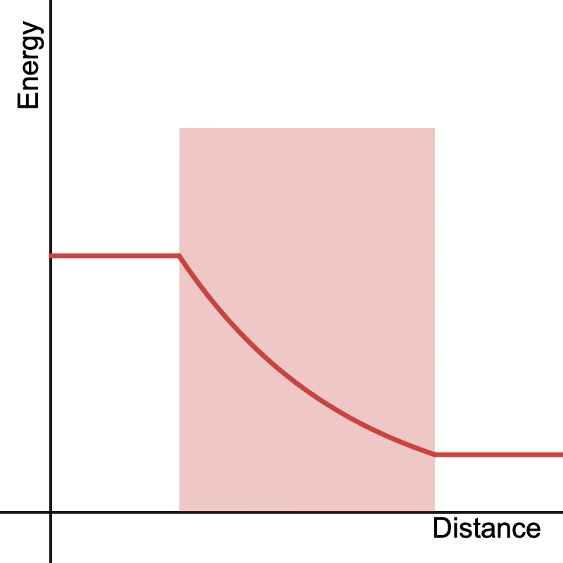
For those unfamiliar, rendering fog boils down to simulating the behaviour of light as it passes through a medium. The simplest behaviour we can model and the one we’re going to focus on is absorption, or the loss of light energy. In basic terms, the more ‘stuff’ that light has to pass through, the more energy it loses.
A light ray loses energy as it travels through a medium (shaded region).
The ratio of outgoing light to incoming light after a given ray passes through a medium is called the transmittance, its value defined as:
Where is the amount of light entering the medium and is the amount coming out. The relationship between the density of the medium and transmittance is described by the Beer-Lambert Law. The equation is:
Where is the total density encountered by the light path going through the medium. Once we have the transmittance, we can just multiply it by to find out how much outgoing light reaches us through the ray. If the medium is just an area of constant density , then simply evaluates to the length of the portion of the light ray passing through the medium times the density:
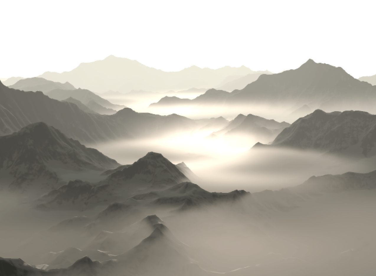
This is more or less the approach the approach used to render simple distance fog in games. Sometimes the Beer-Lambert Law is foregone completely and just the total density along the ray is used to fade objects in the distance. Either way this approach not only assumes a medium of constant density, but that the medium itself covers the entire viewable area.
An example of basic exponential distance fog.
By constraining our medium within a bounded region we can give ourselves a bit more flexibility on the appearance of fog within a scene. The simplest approach is to use primitives such as planes, spheres or boxes as bounding volumes. By determining the intersection of our view ray with these primitives we can find the length of the ray through the volume and calculate the total density using the same formula, once again assuming a constant density within the entire primitive.
Spheres, boxes, and planes can be used to bound regions of fog.
I won’t cover ray-primitive intersection here as it’s beyond the scope of this post and there are loads of resources describing efficient algorithms to do this already. Inigo Quilez has a number of great examples on how to implement these on his website.
Heterogenous Volumes
In reality it’s rare that we can take a medium’s density as constant throughout its entire area, especially when it comes to clouds or smoke. When a medium has a non-constant density we say that it is heterogenous. A greater range of effects can be simulated if we take this into account when rendering. Unfortunately this can complicate the equation quite a bit. Now is no longer a simple product but an integral over the light ray:
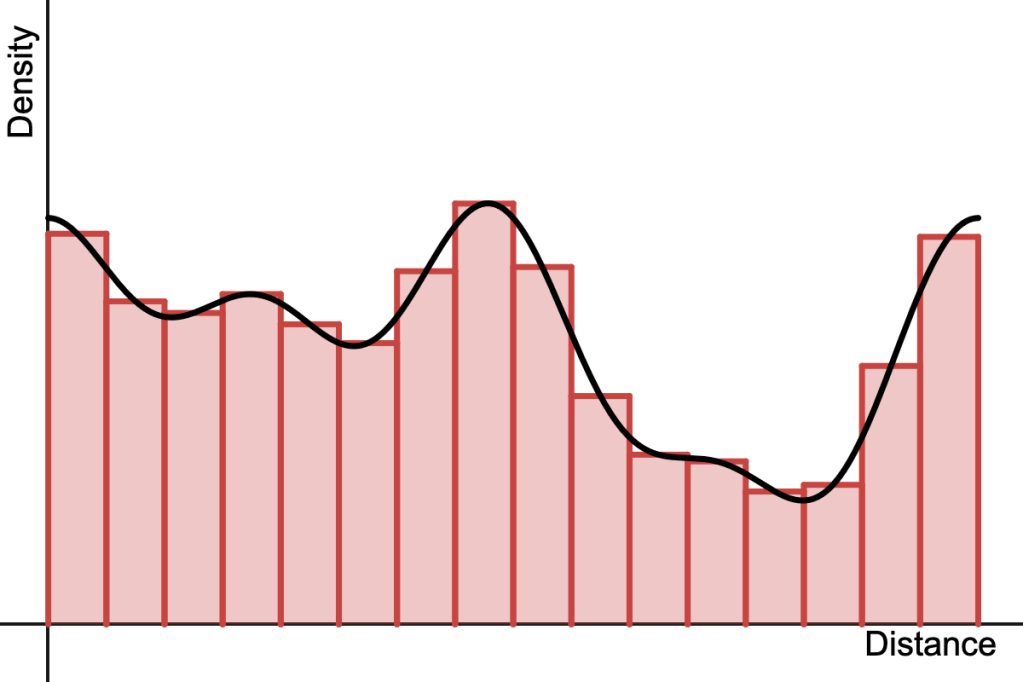
Here, and are the start and end points of the portion of the ray passing through the bounding volume, respectively. The function describes the density of the medium at a given point in space . Because not all functions have a closed-form solution for their integral, we often resort to numerical methods to evaluate it, i.e. moving along the ray in small steps and adding up the area of rectangular ‘slices’ of density along the way.
The integral of an arbitrary function can be approximated by adding up the area of lots of small rectangular slices.
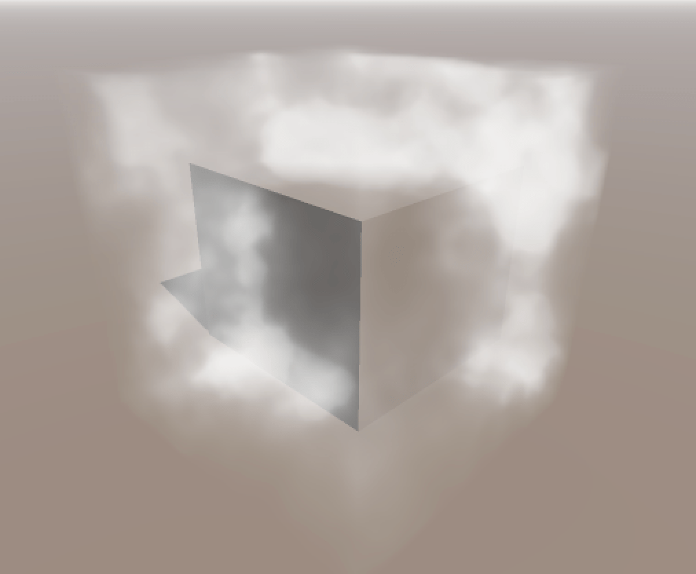
This is effectively what ray-marching does and is pretty much the bread and butter of modern volume rendering. It’s extremely flexible – we don’t care what the density function is, and in fact we may not even know what it is, but as long as we can sample it at arbitrary points (e.g. via a volume texture) we can numerically evaluate the integral.
Ray-marching can be used to render volumes of fog with varying density.
Ray-marching does have its drawbacks however, most notably in the form of aliasing as a result of using too few samples to approximate the integral. While analytic solutions are less flexible, they will never alias and are often faster to compute, which is good motivation for finding analytic expressions for different types of media.
Radial Functions
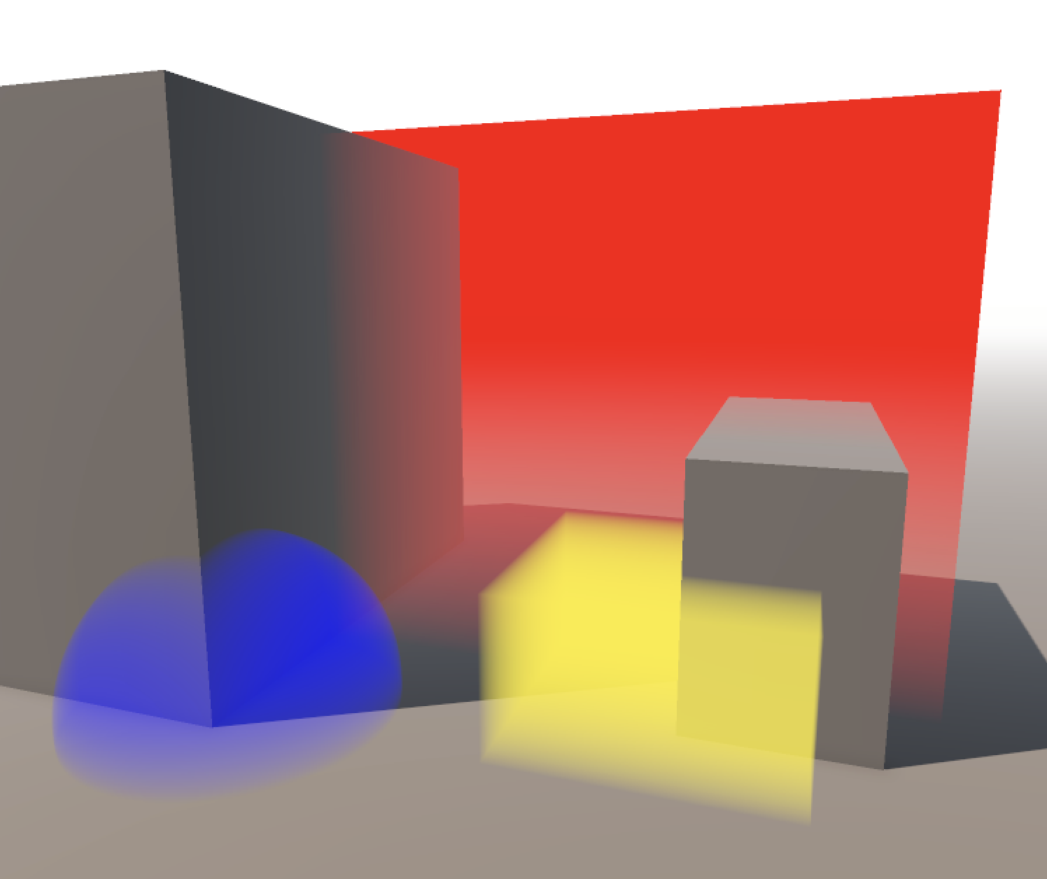
A function that depends on the distance of some point relative to the origin can be considered a radial function. These are nice as they’re often simple to work with and let us define volumes where the density varies over a region. By combining many of these radial density functions we can create more complex fog- or smoke-like effects.
Many radial density functions can be combined to create regions of fog with varying density.
Getting the integral along a line segment is not too difficult for simple functions. Recall that a radial function is dependent on the distance of a point to the centre, which for the sake of simplicity we’ll take to be the point at zero. So the distance is simply:
The equation for a point on a ray with origin and direction at a distance is given by:
So the distance to any point along the ray can be expressed as:
Where:
For a given radial function we can rewrite it in terms of to get a new function that we can (hopefully) integrate. For a more intuitive visual understanding, consider the new function as one that describes the change in density through a cross-section of the original function.
The integral along a ray can be interpreted as the area under the cross-section of the density function (shaded region).
We can apply linear transformations to the ray origin and direction to place arbitrary scaled and rotated volumes anywhere in space without having to change any of the following calculations. This is done by multiplying the ray equation by a transformation matrix in the following way, yielding the transformed ray origin and direction and :
All that’s left is to find the antiderivative of our new function and evaluate it at the limits corresponding to the start and end of the ray. If is the antiderivative of , then:
However, it’s possible that we run into issues with numerical precision when the ray origin is far away from the primitive. We can fix this by moving to the beginning of the interval at , then setting new limits at 0 and , reducing the equation to:
Now I’m going to go through a few radial functions and find the antiderivative of the density along a given ray. You know – for fun!
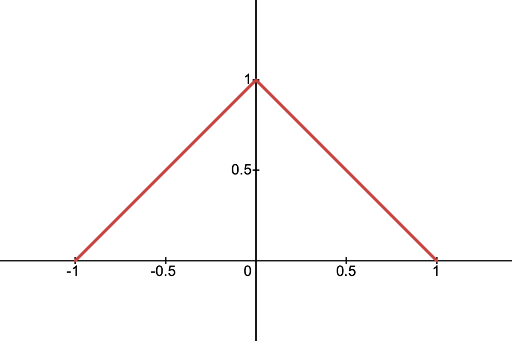
Linear Density
This function corresponds to a triangular function in 1D or a cone in 2D. It’s described by the following equation:
Using the same logic as above, we can define the function for the density along an arbitrary cross-section, which we’ll call :
To find the antiderivative start by pulling out the constant and completing the square:
Then by setting:
We can use the following identity:
Which gives us the final equation, still using and for brevity:
It might be a good idea to add a small offset to the value inside the logarithm, avoiding precision errors near 0. Here’s what all that looks like in code:
float antiderivativeLinear(float a, float b, float c, float t)
{
    float u = t + b / a;
    float v = (b * b - a * c) / (a * a);
    float radical = sqrt(u * u + v);

    return t - sqrt(a) * (u * radical - v * log(0.001f + u + radical)) / 2.0f;
}
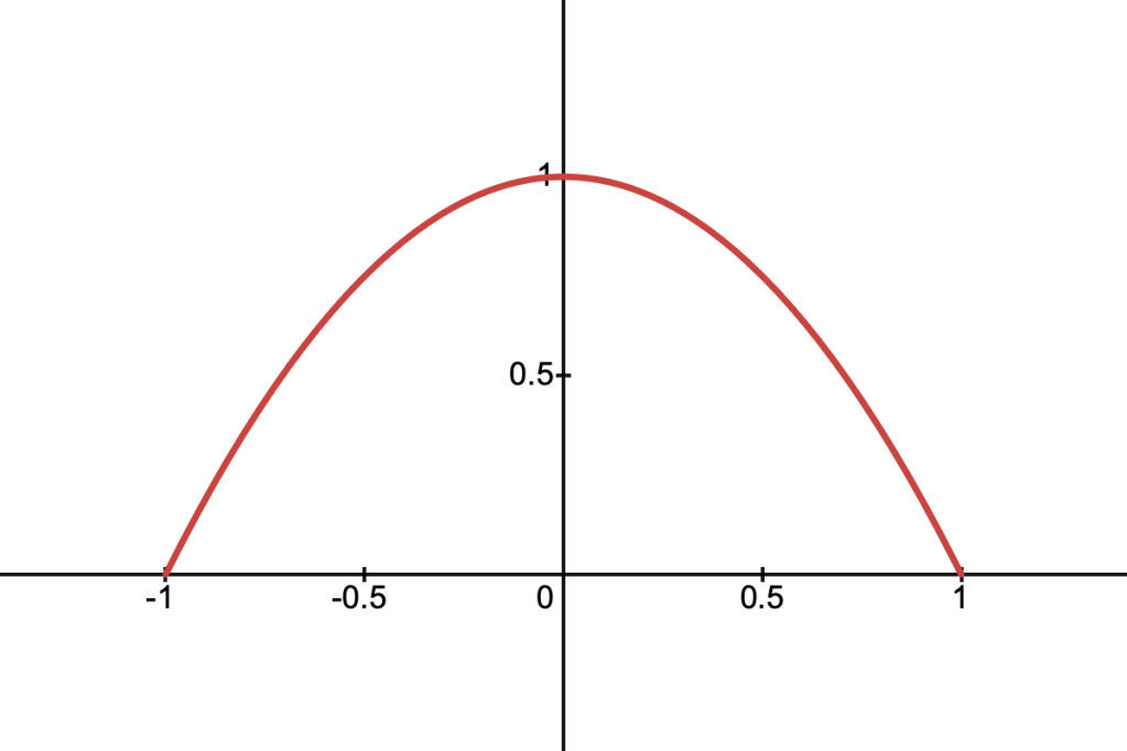
Quadratic Density
This function resembles a parabola and is described by:
Its cross-section along a ray is given by:
Which is nice because we don’t have to deal with any square roots. The equation is a quadratic polynomial in and the antiderivative is easy to solve for:
float antiderivativeQuadratic(float a, float b, float c, float t)
{
    return t * (t * (t * a / -3.0f - b) - c + 1.0f);
}
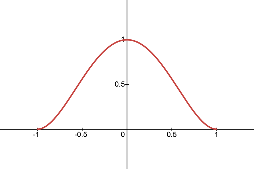
Quartic Density
This function is given by:
And its cross-section along a ray is:
This function is particularly nice because its derivative is zero at the boundaries, similar to smoothstep. The cross-section is a quartic polynomial in t, and the antiderivative is also easy to find:
float antiderivativeQuartic(float a, float b, float c, float t)
{
    return
        t * (t * (t * (t * (a * a * t / 5.0f + a * b) +
        (2.0f * b * b + a * c - a) * 2.0f / 3.0f) +
        (b * c - b) * 2.0f) + (c * c - 2.0f * c + 1.0f));
}
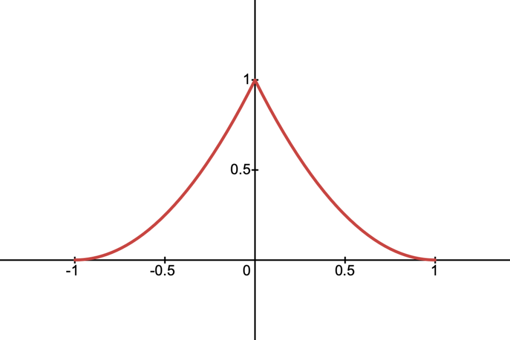
Spiky Density
This is a density function which peaks sharply in the centre and falls off smoothly to zero at the boundaries. It’s defined as:
It’s cross-section is given by:
To find the antiderivative, start by expanding out the brackets:
We can deal with the term the same way we did with the linear density function. The rest of the terms are straightforward. This gives us:
Where once again:
float antiderivativeSpiky(float a, float b, float c, float t)
{
    float u = t + b / a;
    float v = (b * b - a * c) / (a * a);
    float radical = sqrt(u * u - v);

    return
        t * (t * (t * a / 3.0f + b) + c + 1.0f) -
        sqrt(a) * (u * radical - v * log(0.001f + u + radical));
}
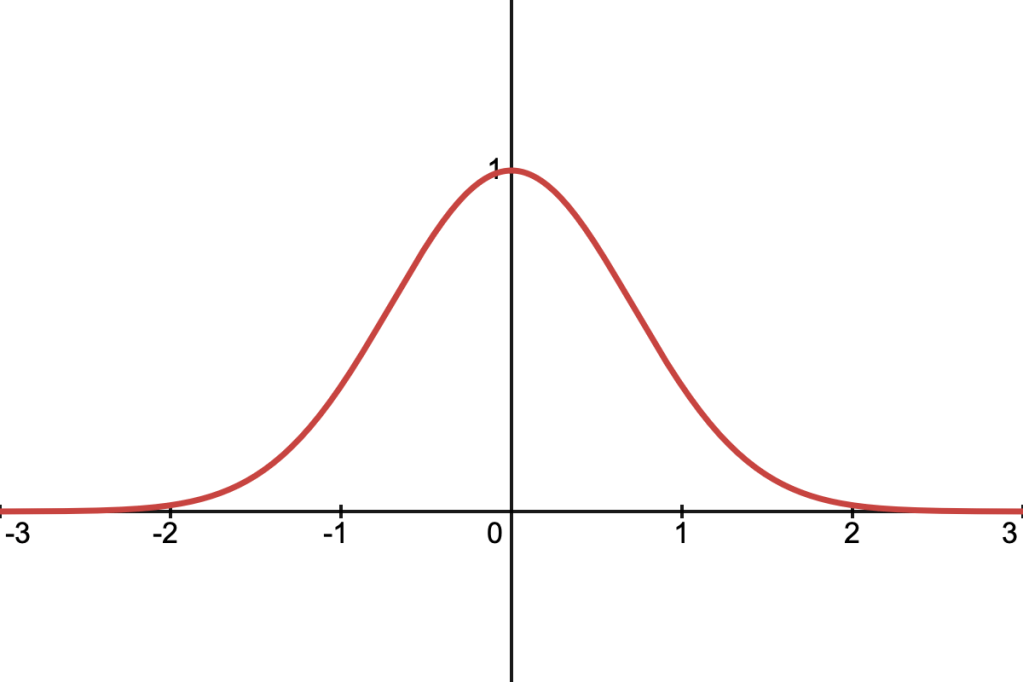
Gaussian Density
This is the well-known Gaussian function, defined as:
It’s cross-section along a ray is:
To find the antiderivative we need to use a function known as the error function, defined as:
To start, we can complete the square in the exponent, which lets us pull out some constant terms from the main integral:
Now we’ll rearrange the exponent so that it’s in the form :
Which lets us use the following substitution:
Yielding:
And after substituting back into our original equation, we arrive at the following solution:
The Gaussian is the only function we’ve covered that doesn’t fall to 0 when , rather it approaches 0 as goes to infinity. In practice it’s often enough to scale and by a constant factor until the discontinuity isn’t noticeable.
// Approximation of erf.
float erf(z)
{
    float az = abs(z);

    return
        sign(z) * (1.0f - 1.0f / pow(1.0f + az * (0.278393f + az *
        (0.230389f + az * (0.000972f + az * 0.078108f))), 4.0f));
}

float antiderivativeGaussian(float a, float b, float c, float t)
{
    float sqrtA = sqrt(a);

    return sqrt(PI) * exp(b * b / a - c) * erf((a * t + b) / sqrtA) / (2.0f * sqrtA);
}
Extra Stuff
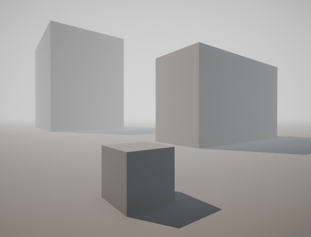
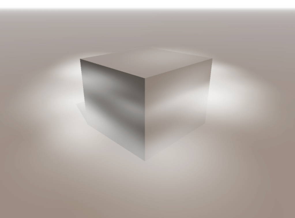
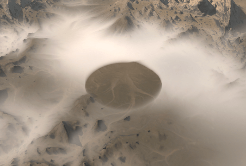
One thing I’ve left out is how to make these volumes respond convincingly to light and shadow. Unfortunately the full equation describing this physical behaviour is too complex to solve analytically. However, a quick hack is to apply a very simple shading model to each individual primitive in the hopes that, as a whole, the medium appears to react to light as we expect it to.
Convincing lighting effects can be achieved using a relatively simple lighting model for each fog primitive.
Representing fog as a collection of primitives opens up some neat possibilities as well. For example, it shouldn’t be too hard to hook these primitives up to a particle system to achieve dynamic or animated fog effects. If we want to be clever we can also use boolean operations to create more complex bounding volumes. This could be used to produce a simple fog of war effect for instance.
Regions of fog can be ‘cut out’ using boolean operations.
I hope you’ve found this technique interesting and find some potential uses for it in your projects. If you’d like a visualisation of all these density functions along with their source code, please take a look at this Shadertoy implementation I put together. Thanks for reading!
In this short post I want to explore a simple and hopefully intuitive geometric interpretation of a common vector operation; the 3D cross product.
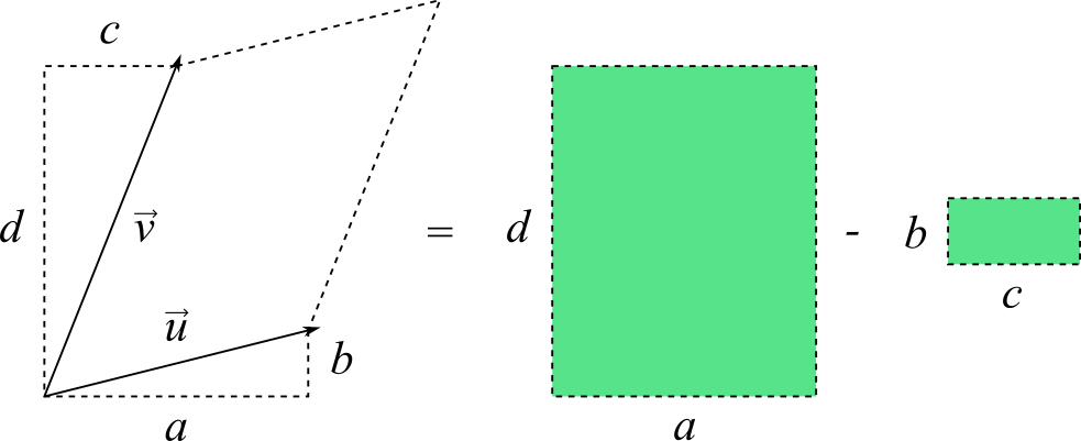
We’ll start by breaking down a somewhat related operation in 2D, sometimes called the perpendicular dot product or just perp dot product. It describes the area of a parallelogram spanned by two vectors and , and is given by the determinant of a 2×2 matrix:
One way to interpret this is that we are subtracting the area of the rectangle from the area of rectangle
The perp dot product can be interpreted as the difference of two rectangles.
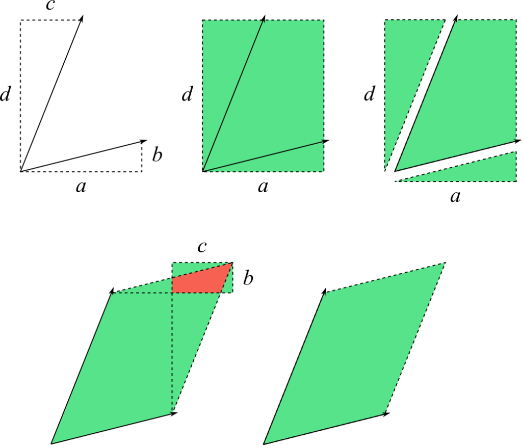
We can put together a simple visual proof by cutting out and rearranging portions of the larger rectangle to show that the smaller rectangle simply cancels out the extra and overlapping areas:
Subtracting the smaller rectangle compensates for the extra area introduced by rectangle . The area highlighted in red indicates an overlap between the parallelogram and .
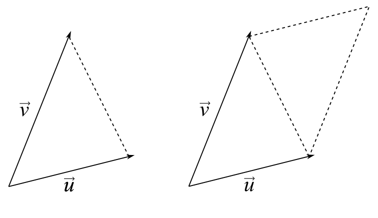
Notice that the area of a triangle with two sides given by the vectors and is exactly half the area of the associated parallelogram. We’ll revisit this property soon.
The vectors and define a triangle as well as a parallelogram of exactly twice the triangle’s area.
In Three Dimensions
We can take the geometric interpretation of the perp dot product to get a more intuitive understanding of the 3D cross product, albeit with a few more steps. The cross product of two vectors and returns another vector whose magnitude describes the area of the parallelogram spanned by and in :
Notice that the cross product operation can be interpreted as three separate perp dot products describing the projection of our original parallelogram onto each of the three coordinate planes. For example, the operation gives the area of the original parallelogram after being projected onto the plane.
The projection of the 3D parallelogram in green onto the bottom plane produces the 2D parallelogram in blue.
The next step is to intuit what it means to take the magnitude of a vector whose components represent the areas of these projected parallelograms. Recall the formula for taking the magnitude of a 3D vector :
This looks like the formula for Euclidean distance, which is derived from the Pythagorean theorem most of us are familiar with. Just to quickly recap, Pythagoras’ theorem states that the squared length of the hypotenuse of a right angled triangle is given by the sum of squared lengths of the legs, and .
Or, in terms of the length :
If we choose to express as a 2D vector , notice how the projection of onto each of the two coordinate axes themselves form a right angled triangle.
Thus, by the Pythagorean theorem:
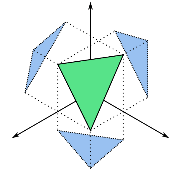
It turns out that this actually generalises to higher dimensions. If we take a triangle in 3D, project it onto each of the three coordinate planes and find the area of each projected triangle, the sum of squares of those areas is equal to the squared area of the original triangle!
The 3D triangle in green is projected onto each of the three coordinate planes, producing three 2D triangles shown in blue.
We can show that this is true by taking what we know about the perp dot product and Pythagoras’ theorem to get the area of a parallelogram just as we would by using the cross product. Let be a triangle in which we express in terms of two vectors representing the edges and . Earlier we established that the area of a triangle is half that of its associated parallelogram, which can be found by using the perp dot product for a parallelogram in . Take the area of each triangle resulting from the projection of onto each coordinate plane and plug them into Pythagoras’ theorem:
We can factor and simplify to take the term out of the square root:
Which we find is equivalent to the following according to the definition of the cross product:
Double the result and you have the area of the parallelogram spanned by and .
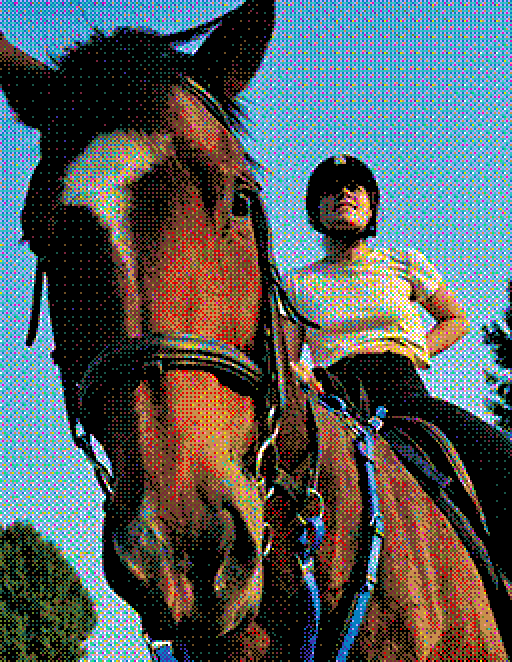
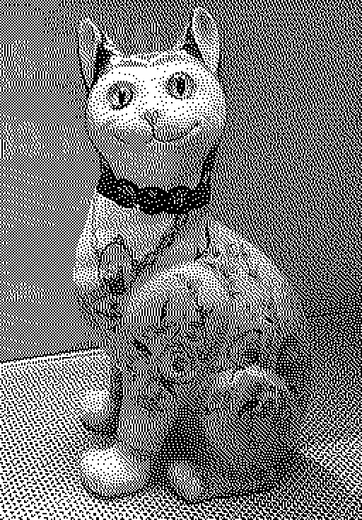
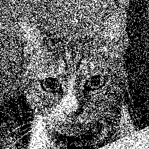
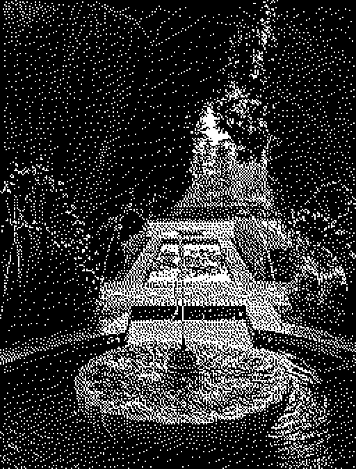
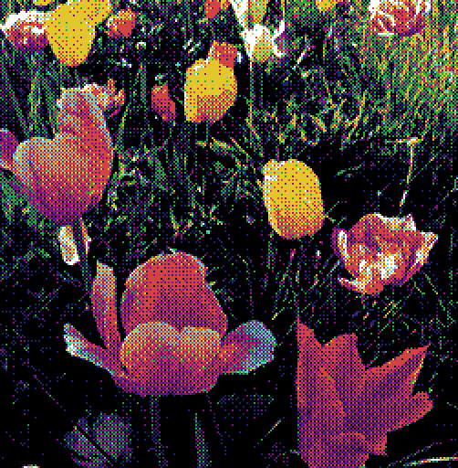
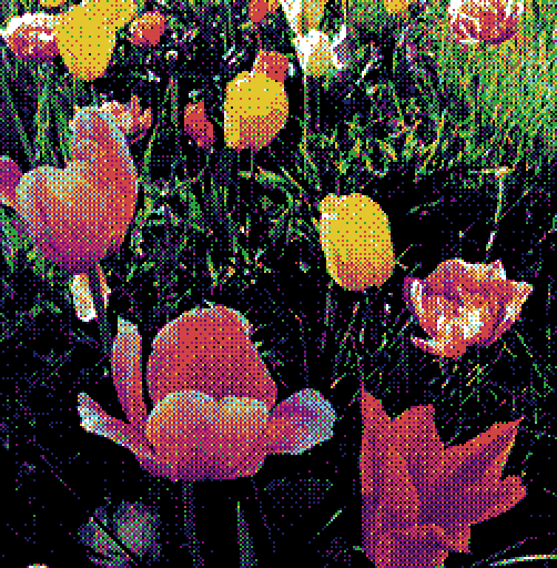
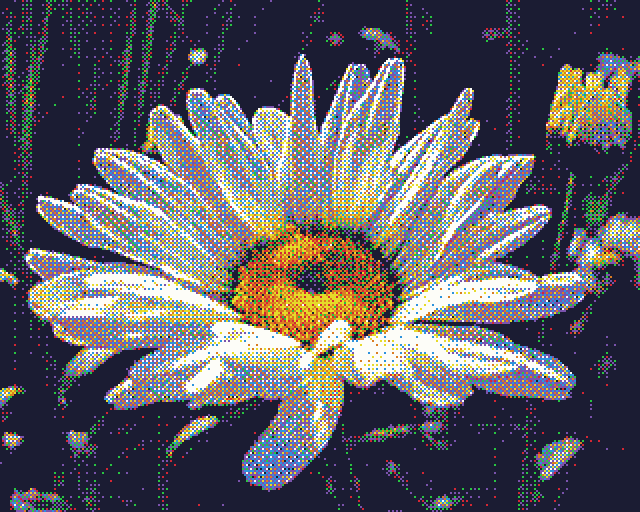
Hello. I have recently been spending a lot of time dithering. In image processing, dithering is the act of applying intentional perturbations or noise in order to compensate for the information lost during colour reduction, also known as quantisation. In particular, I’ve become very interested in a specific type of dithering and its application to colour palettes of arbitrary or irregular colour distributions. Before going into detail however, let’s briefly review the basics of image dithering.
Dithering in its simplest form can be understood by observing what happens when we quantise an image with and without modifying the source by random perturbation. In the examples below, a gradient of 256 grey levels is quantised to just black and white. Note how the dithered gradient is able to simulate a smooth transition from start to end.
An example of dithering using random noise. Top to bottom: original gradient, quantised after dithering, quantised without dithering.
While this is immediately effective, the random perturbations introduce a disturbing texture that can obfuscate details in the original image. To counter this, we can make some smart choices on where and by how much to perturb our input image in an attempt to add some structure to our dither and preserve some of the lost detail.
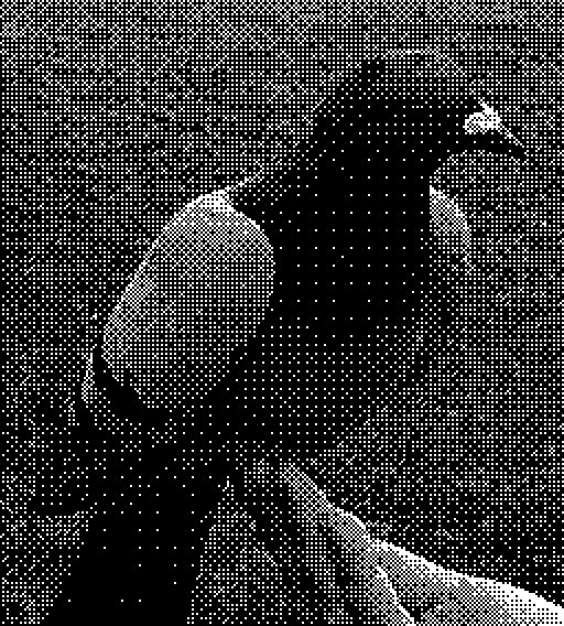
Ordered Dithering
Instead of perturbing each pixel in the input image at random, we can choose to dither by a predetermined amount depending on the pixel’s position in the image. This can be achieved using a threshold map; a small, fixed-size matrix where each entry tells us the amount by which to perturb the input value , producing the dithered value . This matrix is tiled across the input image and sampled for every pixel during the dithering process. The following describes a dithering function for a 4×4 matrix given the pixel raster coordinates :
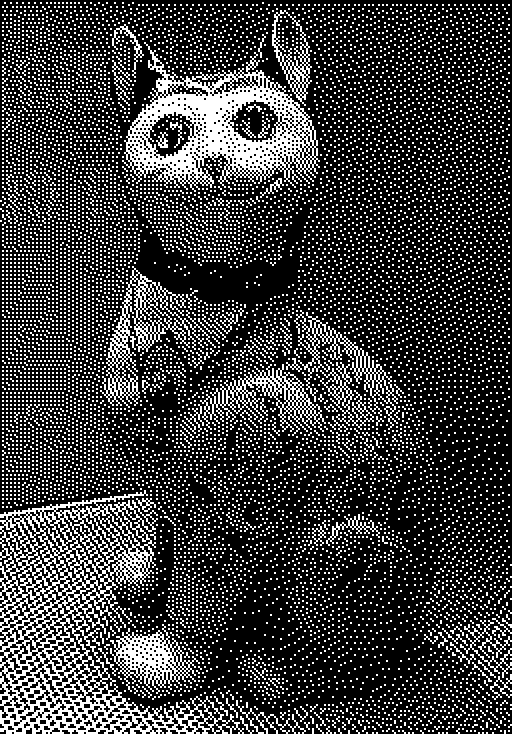
Comparison between random dithering and ordered dithering. Left to right: random, ordered.
We can see that the threshold map distributes perturbations more optimally than purely random noise, resulting in a clearer and more detailed final image. The algorithm itself is extremely simple and trivially parallelisable, requiring only a few operations per pixel.
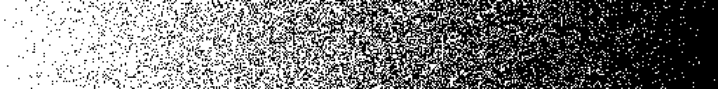
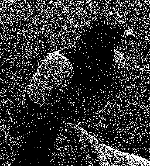
Error-Diffusion Dithering
Another way to approach dithering is to analyse the input image in order to make informed decisions about how best to perturb pixel values prior to quantisation. Error-diffusion dithering does this by sequentially taking the quantisation error for the current pixel (the difference between the input value and the quantised value) and distributing it to surrounding pixels in variable proportions according to a diffusion kernel . The result is that input pixel values are perturbed just enough to compensate for the error introduced by previous pixels.
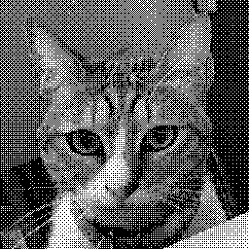
Comparison between error-diffusion dithering and ordered dithering. Left to right: error-diffusion, ordered.
Due to this more measured approach, error-diffusion dithering is even better at preserving details and can produce a more organic looking final image. However, the algorithm itself is inherently serial and not easily parallelised. Additionally, the propagation of error can cause small discrepancies in one part of the image to cascade into other distant areas. This is very obvious during animation, where pixels will appear to jitter between frames. It also makes files harder to compress.
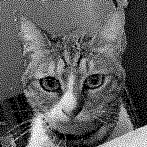
An animated sequence quantised using error-diffusion dithering. Note the jittering artifacts present in the background.
Palette Quantisation
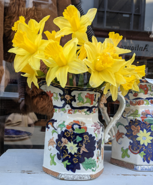
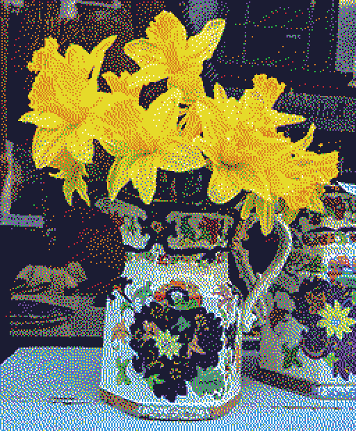
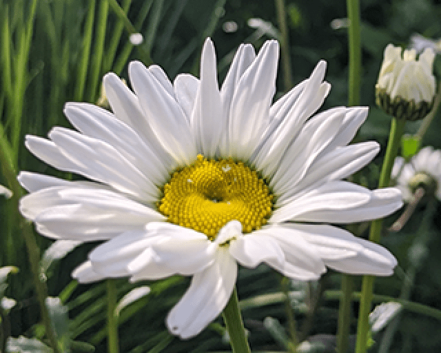
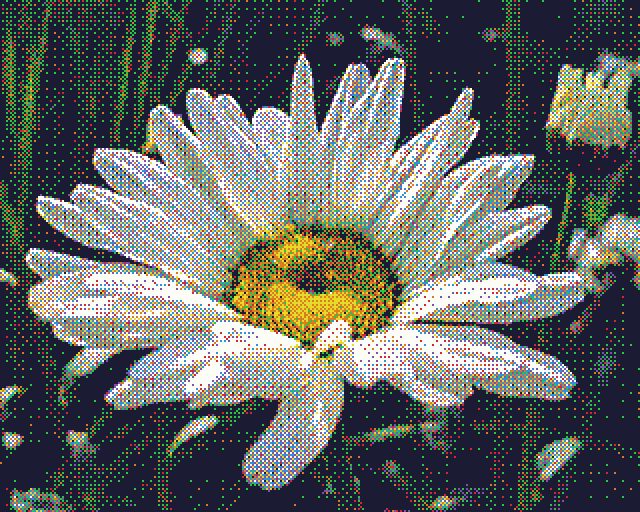
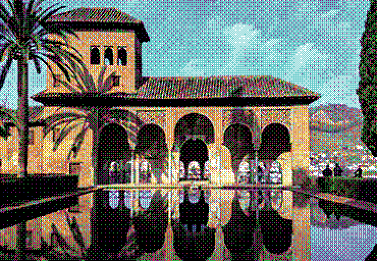
Moving beyond just black and white towards full-colour variable palettes presents another set of problems. Taking the methods presented above and quantising an image using an arbitrary colour palette reveals that error-diffusion is also better at preserving colour information when compared to ordered dithering.
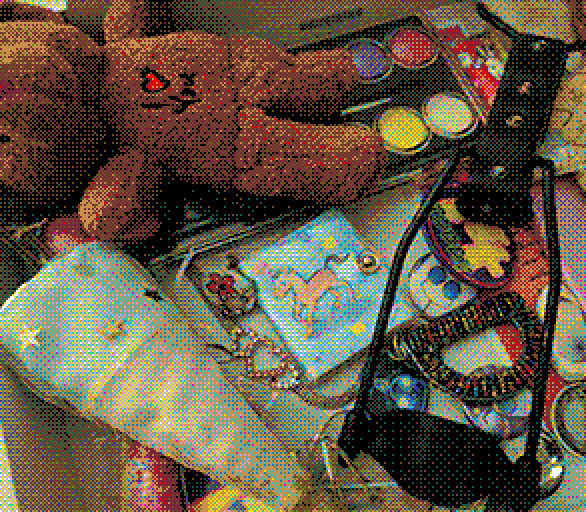
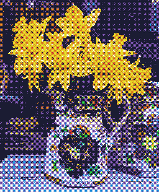
Comparison of error-diffusion vs ordered dithering using an 8-colour irregular palette. Left to right: original image, error-diffusion, ordered.
Intuitively, it’s not too difficult to understand why this is the case. Remember that error-diffusion works in response to the relationship between the input value and the quantised value. In other words, the colour palette is already factored in during the dithering process. On the other hand, ordered dithering is completely agnostic to the colour palette being used. Images are perturbed the same way every time, regardless of the given palette.
Regular vs Irregular Palettes
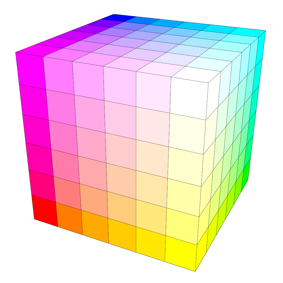
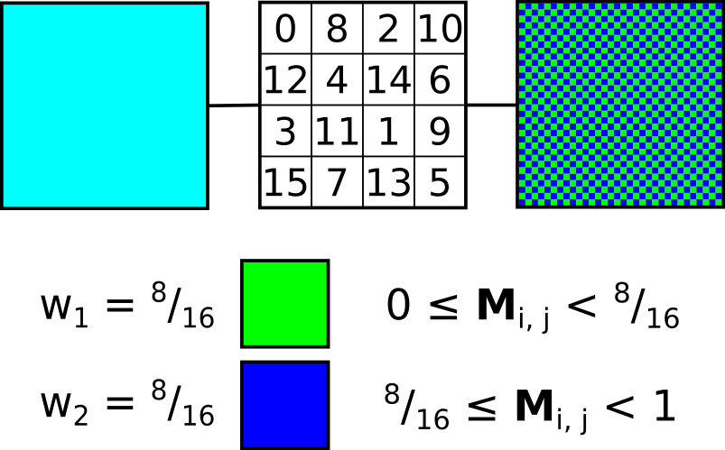
Under certain circumstances, it’s possible to modify ordered dithering so that it can better handle colour information. This requires that we use a palette that is regularly distributed in colour space. A regular palette is composed of all possible combinations of red, green and blue tristimulus values, where each colour component is partitioned into a number of equally spaced levels. For example, 6 levels of red, green and blue totals 6³ = 216 unique colours, equivalent to the common web-safe palette.
Visual representation of an RGB colour cube that has been equally divided into 216 coloured boxes (6 levels along each axis).
This time, before we perturb the input image, we take the value given by the threshold matrix and divide it by , where is the number of levels for each colour component. As a result, each pixel is perturbed just enough to cover the minimal distance between two colours in the palette. Since the entire palette is evenly distributed across colour space, we only need to modify the range of perturbation along each axis. The dithering equation then becomes:
The whole algorithm can be expressed in psuedocode like so:
for each pixel in image let value = value in threshold matrix at (x, y) let offset = pixel + (value - 0.5) * (1.0 / number oflevels) set pixel as closest colour to offset
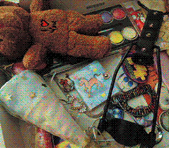
Comparison between error-diffusion and ordered dithering using an 8-colour regular palette. Left to right: error-diffusion, ordered.
By appropriately scaling the perturbation amount for each colour channel separately, we can also extend this to work with palettes where is different for each colour component, provided that they are still regularly spaced. Unfortunately, the less regular the palette is, the less effective this technique becomes. If we wish to leverage the strengths of ordered dithering for use with irregular or arbitrary palettes, a more general solution is needed.
The Probability Matrix
Another way to look at our threshold matrix is as a kind of probability matrix. Instead of offsetting the input pixel by the value given in the threshold matrix, we can instead use the value to sample from the cumulative probability of possible candidate colours, where each colour is assigned a probability or weight . Each colour’s weight represents it’s proportional contribution to the input colour. Colours with greater weight are then more likely to be picked for a given pixel and vice-versa, such that the local average for a given region should converge to that of the original input value. We can call this the N-candidate approach to palette dithering.
A simple demonstration of the use of a probability matrix to select from two candidate colours. In this case, both colours contribute equally to the initial input colour. The normalised threshold matrix value at for a given pixel is compared against the cumulative probability of each candidate.
This approach shares a lot in common with the idea of multivariate interpolation over scattered data. Multivariate interpolation attempts to estimate values at unknown points within an existing data set and is often used in fields such as geostatistics or for geophysical analysis like elevation modelling. We can think of our colour palette as the set of variables we want to interpolate from, and our input colour as the unknown we’re trying to estimate. We can borrow some ideas from multivariate interpolation to develop more effective dithering algorithms.
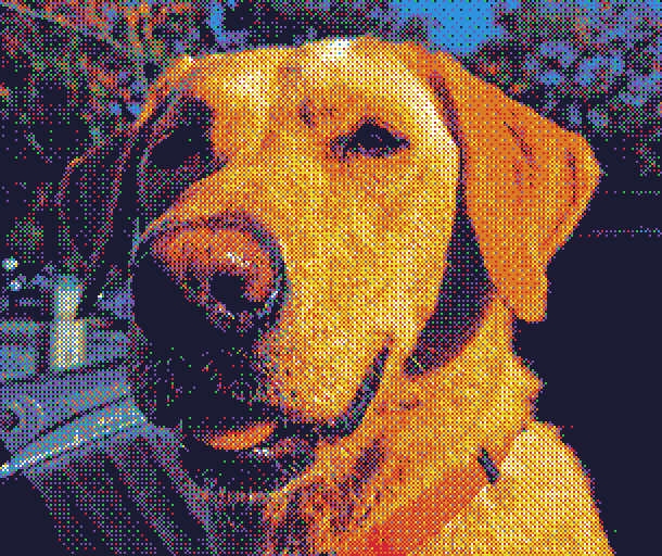
N-Closest Algorithm
The N-closest or N-best dithering algorithm is a straightforward solution to the N-candidate problem. As the name suggests, the set of candidates is given by the closest palette colours to the input pixel. To determine their weights, we simply take the inverse of the distance to the input pixel. This is essentially the inverse distance weighting (IDW) method for multivariate interpolation, also known as Shepard’s method. The following pseudocode sketches out a possible implementation:
for each pixel in image let sum of weights = 0.0 let list of candidates = N closest colours to pixel for eachcandidate in list ofcandidates candidate.weight = 1.0 / distance to candidate sum of weights += candidate.weight for eachcandidate in list ofcandidates candidate.weight /= sum of weights let seed = value in threshold matrix at (x, y) let sum = 0.0 for eachcandidate in list of candidates sum += candidate.weight if seed < sum set pixel as candidate process next pixel
One by-product of weighing the candidates by their distance is that the resulting output image is prone to false contours or banding. Increasing reduces this effect at the cost of added granularity or high frequency noise due to the introduction of ever more distant colours to the set. I recommend taking a look at the original paper if you’re interested in learning a bit more about the algorithm[1].
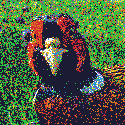
Comparison of N-closest dithering using an 8-colour irregular palette. Left to right: .
Note that IDW often includes a variable exponent that is applied to the distance before taking the inverse. For a given distance , the weight of the candidate becomes:
As you might expect, the result of this is that colours which lie closer to the input pixel are given a greater proportion of the total influence with ever-increasing values of . This is not mentioned in the cited paper but it might be nice to consider for your own implementation.
N-ConvexAlgorithm
Instead of taking the nearest candidates to , we can look for a set of candidates whose centroid is close to . The N-convex algorithm works by finding the closest colour to a given target colour for iterations, where the target is first initialised to be equal to the input pixel. Every iteration the closest colour added to the candidate list, and the quantisation error between it and the original input pixel is added to the target.
for eachpixel in image let goal = pixel do n times candidate[n] = closest colour to goal mark candidate[n] as used goal += pixel - candidate[n]
If this sounds familiar to you, it’s because this method works very similarly to error-diffusion. Instead of letting adjacent pixels compensate for the error, we’re letting each successive candidate compensate for the combined error of all previous candidates.
Comparison of the N-closest and N-convex algorithms using an 8-colour irregular palette with . Left to right: N-closest, N-convex.
Like the N-closest algorithm, the weight of each candidate is given by the inverse of its distance to the input colour. Because of this, both algorithms produce output of a similar quality, although the N-convex method is measurably faster. As with the last algorithm, more details can be found in the original paper[2].
The Linear Combination
If we think about this algebraically, what we really want to do is express the input pixel as the weighted sum of palette colours. This is nothing more than a linear combination of palette colours with weights :
Note however that depending on as well as the distribution of colours in the palette, there may not always be an exact solution for any given . Instead we’ll say that we want to minimise the absolute error between and some linear combination , or .
As it stands, inverse distance weighting is not very good at minimising this error. Another approach is needed if we want to improve the image quality.
Thomas Knoll’s Algorithm
Like the N-convex algorithm, this algorithm attempts to find a set of candidates whose centroid is close to . The key difference is that instead of taking unique candidates, we allow candidates to populate the set multiple times. The result is that the weight of each candidate is simply given by its frequency in the list, which we can then index by random selection:
for eachpixel in image let goal = pixel do n times candidate[n] = closest colour to goal goal += pixel - candidate[n] let seed = random integer from 0 to n set pixel as candidate[seed]
This algorithm attempts to minimise numerically. Because of this, the quality of the dither produced by Knoll’s algorithm is much higher than any other of the N-candidate methods we have covered so far. It is also the slowest however, as it requires a greater per-pixel to be really effective. More details are given in Knoll’s now expired patent[3]. I have put together a GPU implementation of Knoll’s algorithm on Shadertoy here.
Comparison between Thomas Knoll’s algorithm and the N-convex algorithm, using an 8-colour irregular palette. Left to right: original image, Knoll, N-convex ().
Barycentric Coordinates
Another way to approach the linear combination is to look at it geometrically. This is where the idea of barycentric coordinates can help. A barycentric coordinate system describes the location of a point as the weighted sum of the regular coordinates of the vertices forming a simplex. In other words, it describes a linear combination with respect to a set of points, where in -dimensional space.
The barycentric coordinates of are derived from the areas of sub-triangles .
The weight of each term is given by the proportion of each sub-triangle area with respect to the total triangle area . Algebraically, this can be expressed like so:
Knowing this, we can modify the N-Convex algorithm covered earlier such that the candidate weights are given by the barycentric coordinates of the input pixel after being projected onto a triangle whose vertices are given by three surrounding colours, abandoning the IDW method altogether1. This results in a fast and exact minimisation of , with the final dither being closer in quality to that of Knoll’s Algorithm.
Comparison between barycentric (triangular) dithering and Knoll’s algorithm using an 8-colour irregular palette. Left to right: barycentric, Knoll.
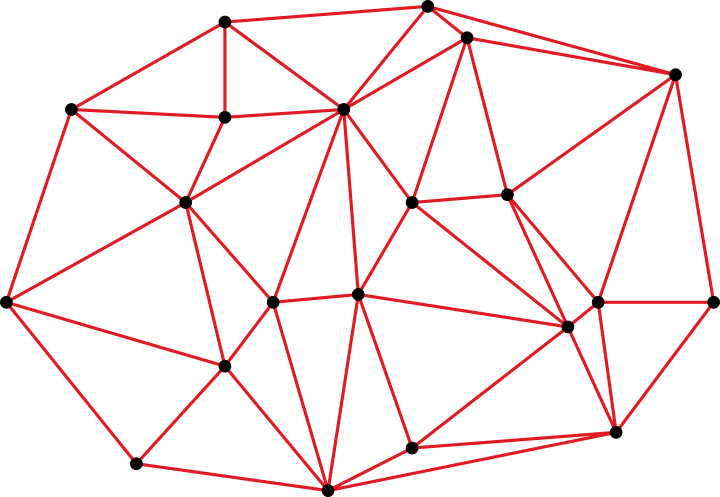
Triangulated Irregular Network
Recall that a barycentric coordinate system is given with respect to a -dimensional simplex, where is no larger than the dimensional space. Given a set of scattered points, it’s possible to create a tessellation of the space by forming simplices from the points, such that any input point that lies within the convex hull of the scattered set can be expressed in terms of the enclosing simplex and its corresponding barycentric coordinates2. This can be understood as a kind of triangulated irregular network (TIN).
An example of a triangulated irregular network. The known data sites (black points) are triangulated to form a convex hull.
While there exist many possible ways to triangulate a set of points, the most common method for TINs is the Delaunay triangulation. This is because Delaunay triangulations tend to produce more regular tessellations that are better suited to interpolation. In theory, we can represent our colour palette as a TIN by computing the 3D Delaunay triangulation of the colours in colour space. The nice thing about this is that it makes finding an enclosing simplex much faster; the candidate selection process is simply a matter of determining the enclosing tetrahedron of an input point within the network using a walking algorithm, and taking the barycentric coordinates as the weights.
Comparison between the TIN, Knoll’s algorithm, and N-convex dithering using an 8-colour irregular palette. Left to right: TIN, Knoll, N-convex (N=4).
If executed well, Delaunay-based tetrahedral dithering can outperform the N-convex method and produce results that rival Knoll’s algorithm. The devil is in the detail however, as actually implementing a robust Delaunay triangulator is a non-trivial task, especially where numerical stability is concerned. The additional memory overhead required by the triangulation structure may also be a concern.
Natural Neighbour Interpolation
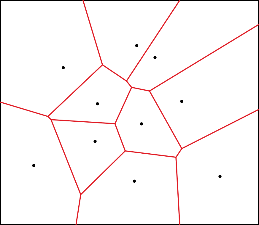
We’ve looked at how we can geometrically find the linear combination using barycentric coordinates, but it is not the only way to do so. Natural neighbour interpolation works by observing what happens when an input point is inserted into a set of points represented by a Voronoi diagram. The Voronoi diagram is simply a partition of space into polygonal regions for each data point, such that any point inside a given region is proximal to its corresponding data point.
Any point within a given Voronoi region is proximal to the data site (black point) associated with that region.
When another data point is inserted and the Voronoi diagram reconstructed, the newly created region displaces the area that once belonged to the old regions. Those points whose regions were displaced are considered natural neighbours to the new point. The weight of each natural neighbour is given by the area taken from the total area occupied by the new region. In 3D, we measure polyhedral volumes instead of areas.
The query point creates a new Voronoi region shown in blue, displacing some of the old regions. The weight of each natural neighbour is derived from the area of the displaced region .
Natural neighbour interpolation has a number of strengths over linear barycentric interpolation. Namely, it provides a smooth or continuous slope between samples3, and is always the same for a given point set, unlike the TIN where the quality of the triangulation can produce biases in the outcome, even in the best case.
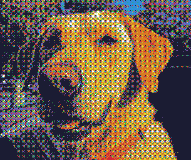
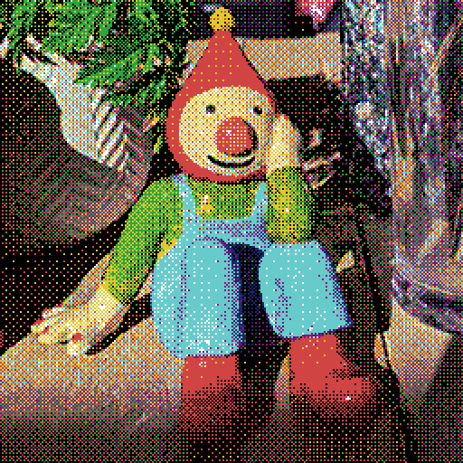
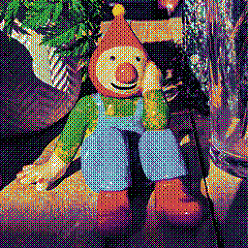
Comparison between TIN and natural neighbour dithering, using a 16-colour irregular palette. Left to right: TIN, Natural Neighbour.
Implementing natural neighbour interpolation implies the construction of a geometric Voronoi diagram, however this is not strictly the case. Since the Delaunay triangulation is the dual graph of the Voronoi diagram, all the information needed to perform natural neighbour interpolation is already implicit within the triangulation itself. Algorithms to determine natural neighbours from the Delaunay triangulation can be found in several papers within the literature[4][5]. Unfortunately the relative complexity of natural neighbour interpolation means that it is slower than barycentric interpolation by a considerable margin.
Joel Yliluoma’s Algorithms
A notable resource on the topic of ordered dithering using arbitrary palettes is Joel Yliluoma’s Arbitrary-Palette Positional Dithering Algorithm. One key difference of Yliluoma’s approach is in the use of error metrics beyond the minimisation of . Yliluoma notes that the perceptual or psychovisual quality of the dither must be taken into account in addition to its mathematical accuracy. This is determined by use of some cost function which considers the relationship between a set of candidate colours. The number of candidates, the particular cost function, and the thoroughness of the selection process itself give rise to a number of possible implementations, each offering varying degrees of quality and time complexity.
Comparison between Knoll’s and Yliluoma’s algorithms using a 16-colour irregular palette. Left to right: Knoll, Yliluoma. The ‘Yliluoma’s ordered dithering algorithm 2‘ variant was used.
Yliluoma’s algorithms can produce very good results, with some variants matching or even exceeding that of Knoll’s. They are generally slower however, except in a few cases.
Tetrapal: A Palette Triangulator
Most of the algorithms described here are quite straightforward to implement. Some of them can be written in just a few lines of code, and those that require a bit more effort can be better understood by reading through the relevant papers and links I have provided. The exception to this are those that rely on the Delaunay triangulation to work. Robust Delaunay triangulations in 3D are fairly complex and there isn’t any publicly available software that I’m aware of that leverages them for dithering in the way I’ve described.
To this end, I have written a small C library for the sole purpose of generating the Delaunay triangulation of a colour palette and using the resulting structure to perform barycentric interpolation as well as natural neighbour interpolation for use in colour image dithering. The library and source code is available for free on Github. I’ve included an additional write up that goes into a bit more detail on the implementation and also provides some performance and quality comparisons against other algorithms. Support would be greatly appreciated!
Appendix I:Candidate Sorting
When using the probability matrix to pick from the candidate set, it is important that the candidate array be sorted in advance. Not doing so will fail to preserve the patterns distinctive of ordered dithering. A good approach is to sort the candidate colours by luminance, or the measure of a colour’s lightness4. When this is done, we effectively minimise the contrast between successive candidates in the array, making it easier to observe the pattern embedded the matrix.
Comparison between an unsorted and a luminance sorted candidate set, using Knoll’s algorithm on an 8-colour irregular palette. Left to right: unsorted, sorted.
If the number of candidates for each pixel grows too large (as is common in algorithms such as Knoll and Yliluoma) then sorting the candidate list for every pixel can have a significant impact on performance. A solution is to instead sort the palette in advance and keep a separate tally of weights for every palette colour. The weights can then be accumulated by iterating linearly through the tally of sorted colours.
sort palette by luminance letweights[palette size] = weight for each colour ... for iin range 0 topalette size - 1 cumulative weight += weights[i] ifcumulative weight < probability value set pixel as palette[i]
Appendix II:Linear RGBSpace
Most digital images intended for viewing are generally assumed to be in sRGB colour space, which is gamma-encoded. This means that a linear increase of value in colour space does not correspond to a linear increase in actual physical light intensity, instead following more of a curve. If we want to mathematically operate on colour values in a physically accurate way, we must first convert them to linear space by applying gamma decompression. After processing, gamma compression should be reapplied before display. The following C code demonstrates how to do so following the sRGB standard:
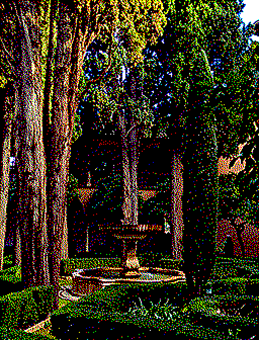
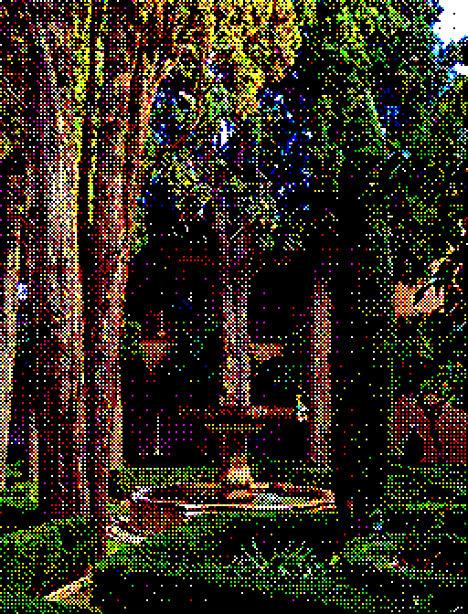
Comparison between error-diffusion dithering in sRGB space and linear RGB space. Left to right: sRGB, linear.
Appendix III: Threshold Matrices and Noise Functions
All of the examples demonstrating ordered dithering so far have been produced using a specific type of threshold matrix commonly known as a Bayer matrix. In theory however any matrix could be used and a number of alternatives are available depending on your qualitative preference. Matrices also don’t have to be square or even rectangular; polyomino-based dithering matrices have been explored as well[6].
The classic Bayer or ‘dispersed-dot’ pattern arranges threshold values in an attempt to optimise information transfer and minimise noise[7]. The matrix dimensions are typically a power of two. The following values describe an 8×8 matrix:
The halftone or ‘clustered-dot’ matrix uses a dot pattern reminiscent of traditional photographic halftoning. Here a diagonal variant of the pattern is given:
The blue noise or ‘void-and-cluster’ dither pattern avoids directional artefacts while retaining the optimal qualities of the Bayer pattern. The Bayer matrix can in fact be derived from the void-and-cluster generation algorithm itself[8].
You can access some tiled blue noise textures in plain text format here. I have also released a small C library for generating these textures.
It’s also possible to abandon the threshold matrix altogether and instead calculate a value for every pixel coordinate at runtime. If the function is simple enough this can be a good and efficient way to break up patterns and create interesting textures.
White noise simply uses a random number generator to produce threshold values.
Interleaved gradient noise is a form of low-discrepancy sequence that attempts to distribute values more evenly across space when compared to pure white noise[9].
The R-sequence is another type of low-discrepancy sequence based on specially chosen irrational numbers[10]. It is similar to interleaved gradient noise but is simpler to compute and possibly more effective as a dither, particularly when augmented with a triangle wave function as demonstrated:
float r_sequence(int x, int y)
{
    float value = fmodf(0.7548776662f * (float)x + 0.56984029f * (float)y, 1.0f);
	return value < 0.5f ? 2.0f * value : 2.0f - 2.0f * value;
}
Footnotes
1 It’s also possible to use 4 candidates per pixel and compute the barycentric coordinates of the resulting tetrahedron, but using 3 candidates forming a triangle is more straightforward. ↑
2 For points outside the convex hull, an acceptable solution is to find the closest point on the surface and determine the barycentric coordinates for that point instead. ↑
3 Strictly speaking, the slope is continuous everywhere except for the data points themselves. ↑
4 A good discussion on luminance and how to calculate it can be found on this stack exchange question. ↑
References
[1] K. Lemström, J. Tarhio & T. Takala: “Color Dithering with n-Best Algorithm” (1996). ↑
[2] K. Lemström & P. Fränti: “N-Candidate methods for location invariant dithering of color images” (2000). ↑
[3] T. Knoll: “Pattern Dithering” (1999). US Patent No. 6,606,166. ↑
[4] M. Sambridge, J. Braunl & H. McQueen: “Geophysical parametrization and interpolation of irregular data using natural neighbours” (1995). ↑
[5] L. Liang & D. Hale: “A stable and fast implementation of natural neighbour interpolation” (2010). ↑
[6] D. Vanderhaeghe & V. Ostromoukhov: “Polyomino-Based Digital Halftoning” (2008). ↑
[7] B. E. Bayer: “An optimum method for two-level rendition of continuous-tone pictures” (1973). ↑
[8] R. Ulichney: “The void-and-cluster method for dither array generation” (1993). ↑
[9] J. Jimenez: “Next Generation Post Processing in Call of Duty: Advanced Warfare” (2014). ↑
[10] M. Roberts: “The Unreasonable Effectiveness of Quasirandom Sequences” (2018). ↑


 of a parallelogram spanned by two vectors
  and
and  , and is given by the
 from the area of rectangle
 and
and  is exactly half the area of the associated parallelogram. We’ll revisit this property soon.
 :
:
 gives the area of the original parallelogram after being projected onto the
  plane.
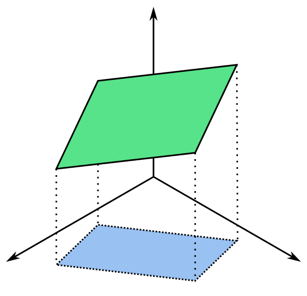

 of a right angled triangle is given by the sum of squared lengths of the legs,
  .
.


 , notice how the projection of
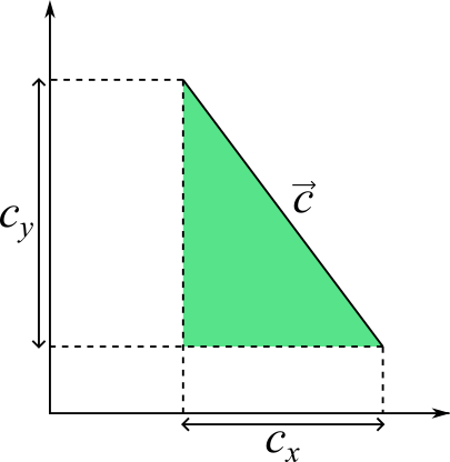

 be a triangle in
  and
and  . Earlier we established that the area of a triangle is half that of its associated parallelogram, which can be found by using the perp dot product for a parallelogram in
  . Take the area of each triangle resulting from the projection of
 term out of the square root:


 where each entry tells us the amount by which to perturb the input value
  . This matrix is tiled across the input image and sampled for every pixel during the dithering process. The following describes a dithering function for a 4×4 matrix given the pixel raster coordinates
  :
:

 . The result is that input pixel values are perturbed just enough to compensate for the error introduced by previous pixels.

 , where
 possible candidate colours, where each colour
  is assigned a probability or weight
  . Each colour’s weight represents it’s proportional contribution to the input colour. Colours with greater weight are then more likely to be picked for a given pixel and vice-versa, such that the local average for a given region should converge to that of the original input value. We can call this the N-candidate approach to palette dithering.

 for a given pixel is compared against the cumulative probability of each candidate.
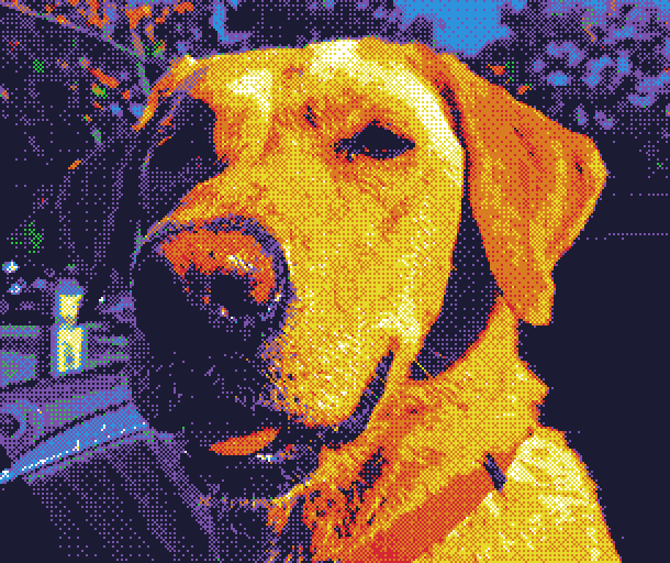
 .
. that is applied to the distance before taking the inverse. For a given distance
  , the weight
  of the candidate becomes:
 . Left to right: N-closest, N-convex.
 , or
, or  .
.
 in
in  -dimensional space.
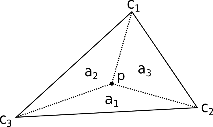
 are derived from the areas of sub-triangles
  .
. with respect to the total triangle area
 , with the final dither being closer in quality to that of Knoll’s Algorithm.
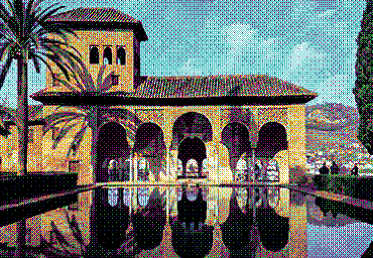

 taken from the total area

 is derived from the area of the displaced region
  .
.